ELSA is an integrated tool for astrophysics researchers. It is meant to serve a bridge between raw data logs taken with the Image Reduction and Analysis Facility (IRAF) and the final, organized tabular data. It was originally designed to analyze emission-line spectrum data from planetary nebulae, but it is also possible to use certain features of ELSA on a host of astronomical objects that produce similar spectra. ELSA integrates much of the latest research in atomic physics and astrophysics, as well new, original methods, to produce sophisticated calculations of ionic and elemental abundances, electron temperatures, and electron densities based on emission line strengths. It also provides facilities for managing and formatting the resultant data for use in research and publications.
ELSA was developed by Matthew D. Johnson and Jesse S. Levitt at Williams College in the summer of 2005. Large portions of it are based heavily on the work of Karen Kwitter at Williams College and Dick Henry at the University of Oklahoma. It borrows widely from the established work of numerous individuals who have developed atomic data and constants for use in applications like these.
What follows is the comprehensive documentation for ELSA. It includes the basic and setup, and operation of the program, as well as a guide for experienced and semi-experienced programmers who wish to modify the code. We would appreciate it if any significant modifications to the code could be brought to our attention, as ELSA is still a work in progress and we wish to include as many as improvements and advances as possible in future versions of the code.
If you find ELSA to be useful to you in your research and analysis, we encourage you to tell us and provide feedback on how future versions could be expanded and improved.
The latest source code and binaries for ELSA can always be found on the website:
http://www.williams.edu/astronomy/research/PN/.
To obtain a working copy of ELSA, there are two options. If you use Mac OS X (PowerPC),
Solaris (SPARC), or Linux (i386), you may download the binaries for your system. These are
pre-compiled for specific system and platform. If you’re not using one of the above, or you prefer to
compile your own binary, obtain the source code distribution. In any case, unpack it as
such:
gunzip elsa-1.0.tar.gz
tar -xvf elsa-1.0.tar
If you’re compiling from souce, you then should be able go into the elsa/src directory and run
make. This will build your elsa binary and place it at the root level of the directory (outside src.
If this seems to have worked correctly, you’re done. Now you will probably want to edit your config
file, elsa.conf, as described in section 3.1.2.
If your system has a non-standard make and isn’t able to deal with the Makefile provided here,
you can build it manually with the following:
gcc -o elsa *.c -lm
Your C compiler may be called cc if your system is old enough not to have the GNU C compiler
(GCC) installed on it. If you experience any severe system-specific problems that prevent you from
compiling or running ELSA, please let us know!
ELSA is designed on and for UNIX systems. Currently there is no version for Windows or other operating systems. It may be possible to compile and run the code on such systems provided that there is sufficient compatibility with the POSIX library calls. In these cases, you will need to make sure that you link against libmath (the -lm option in GCC) or you may experience very strange mathematical behavior.
The source code compiles to a single UNIX binary. This binary will provide an interface to the multiple “tasks” that make up ELSA’s suite of tools. Each task has a specific function and takes specific arguments and parameters (typically names of input and output files, or numerical constants required for the operation the task performs). There is also a general configuration file (called elsa.conf by default) which provides the values of several important global constants and switches that pertain to all tasks in the program, such as the values of Hα and Hβ, the wavelength tolerance threshold, and more. See section 3.2 for descriptions of these run-time configuration variables.
The tasks fall into one of three categories: log merging and management, table generation, and abundance calculation. Log merging and management tasks process the data in splot log files produced by IRAF, and run diagnostics on it to flag unknown wavelengths and measurements with long comments. Table generation tasks will create organized data tables in various table formats after performing corrections for reddening, helium recombination contamination, temperature and density dependence, and Balmer ratio variance. Abundance calculation tasks will compute ionic and elemental abundances, electron temperatures, and electron densities based on line strengths after performing the aforementioned corrections.
ELSA is run from the UNIX command line as such:
elsa [options] [task] [task syntax ...]
The syntax for each task is listed in its respective subsection below.
There are a small number command line options available. In this version, they only control the preferred output format. This version can output in human readable (tab-delimited) format, in the CSV (comma separated value) format suitable for use with tabular data and plotting programs, and in LATEX (with the AASTEX extensions) format. Running elsa -h will print the online help, which shows the list of tasks and command line options present in the current version. As of the time of this writing, the options are:
It is possible to stack options (such as -vc), but as of this version there is no reason to do this as all the options are mutually exclusive. In the event that, for example, two conflicting formatting options are given, the last option given will take precedence. Note that not all output formats are available for all tasks. See the task reference below for more information about possible output formats for specific tasks.
The global configuration file is by default named elsa.conf and will unpack in the same directory as the source code and documentation. Before running ELSA, you should edit the configuration file and make sure that the values in it are acceptable for your data. The configuration file contains comments which explain the values in it. Here are the important parameters you will need to set:
The spec file contains the list of reference wavelengths to be used for table generation and abundance calculation tasks. The format of the file is simple: each line contains a wavelength in angstroms as a floating point value (note that both integers and decimals are acceptable as floating point values) followed by a space, followed by the text description of what ion the wavelength is related to. Everything after the initial space is considered to be this text description. The number of lines in the spec file should not exceed the amount specified by the MaxSpec configuration variable. If it does, lines beyond the specified limit are ignored. Comments and blank lines are not allowed in the spec file, and their presence may cause formatting faults which will prevent ELSA from being able to complete a run.
The “master list” of wavelengths read from this file is used to generate table output, and to generate the data that is passed to the abundance calculation routines. If a wavelength does not appear in the spec file, it will be ignored by ELSA in all table generation and abundance calculation tasks.
See the provided sample “wavelengths.txt” for a guide to creating spec files.
Syntax: splot_merge <file_1> <file_2> [scale] [output_file]
The splot_merge task consolidates two splot log files generated by IRAF into a single log. Raw, unedited logs should work correctly. The expected format of the log files is columns of floating point values. This task will read the files line by line, taking the first column as the wavelength and the third column as the flux. The second column (the continuum level) and all columns after the third are ignored. The task also ignores any line that does not begin with a number (i.e., it will ignore blank lines and “header” lines). Lines beginning with a pound sign (#) are taken to be comments. Comments are preserved throughout all processes in ELSA. All the text after the pound sign is taken to be the comment. The pound sign itself and all leading and trailing whitespace are deleted. All comments are associated with the last valid line of data that was read. In the event of multiple consecutive comments, the strings will be concatenated into a single comment string and associated with the last valid line of data.
The output will be in the same format, although zeroes will be output as placeholders for the continuum level (this will not cause problems when the output log is read, since the continuum level is ignored). Comments will be output prefixed by a pound sign following the line that they refer to. Output is written to the named output_file if it is provided and the file writable. If not, output will be to the standard output. Since this task has a special output format, all command line options about output formats are ignored.
The parameter scale is a floating point value by which all the flux values in file_2 will be multiplied prior to processing. The goal of the scale factor is normalize all the flux values across both files to the same scale (in the event that the instrumentation used to obtain the data produced different scales for different ends of the spectrum). There is no facility in ELSA to calculate the scale factor automatically. The scale factor parameter is optional. If it is not provided, it will be assumed to be 1.0.
After the scale factor has been applied to file_2, this task will iterate through each line in both files. It will find all other lines whose wavelength falls within ± the value of the MaxTolerance configuration variable of the wavelength in question. All such overlaps that are found will cause you to be prompted to select one of the overlapping lines to be written into the output file. This will eliminate all duplicate lines, whether they happen to be in the same file or in different files. The prompt will present you with the wavelength, flux, and comment for you evaluate.
It is recommended that you check the output file against your input files to ensure that your MaxTolerance setting was sufficient to both catch all overlaps, and to prevent finding false overlaps. This task is ultimately intended to produce valid input for the table generation and abundance calculation tasks, which cannot deal with duplicate line matches. Always save original copies of your data.
Syntax: splot_undup <file> [output_file]
The splot_undup task functions very similarly to splot_merge. However, instead of reading its “pool” of data from two files, it only reads it from one. There is, obviously, no need for a scale factor in this case. As in splot_merge, overlapping measurements are located using the MaxTolerance variable and you will be prompted as described in the previous section to choose one of the overlapping measurements. Output is written to the provided output file name, or to standard output if the output file name is not provided or the file is not writable. As is the case with splot_merge, all command line options for output formats are ignored.
Syntax: splot_flag <file> <velocity> [output_file]
The splot_flag task will find measurements in an splot log that do not match any of the reference wavelengths in the spec file. It will also find any measurements that have long associated comment strings, which likely indicates some sort of special narrative remark on the measurement (rather than a standard number of colons to indicate uncertainty).
Matching will occur in the inverse of the normal method. The velocity parameter will be applied as described in section 3.3.1 and the “expected” wavelengths shifted accordingly. The MaxTolerance variable will then be used to determine the upper and lower limits for matching a specific reference wavelength.
Output will be written to the named output file or to standard output if it is not available or not provided. The output will be human readable text in two sections: one for the unknown wavelengths, and one for the long comments.
Syntax: splot_table <file> <velocity> [output_file]
The splot_table task generates a complete table of extinction-corrected line intensities based on an splot log. It takes a single file of input, which must be in the log format described in the previous section. It is strongly recommended that you run splot_merge or splot_undup on your data before attempting to run this task on it; the output from those tasks will (almost) always be compatible with splot_table.
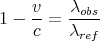
The table generated is based directly on the list of reference wavelengths in the spec file given by the SpecFile configuration variable. This task will systematically walk the list of reference wavelengths and try to match them to measured wavelengths in the log file. Two factors apply in this matching. The first is the velocity parameter passed to the task from the command line. This is the radial velocity of the object in question, in kilometers per second. Based on this parameter, splot_table will determine a wavelength shift and apply it to all wavelengths in the file. The equation for this shift is:
|
| (1) |
Once this shift has been applied, the task will attempt to match λobs instead of λref to measured wavelengths. Matches will be made for measured wavelengths within the limits given by λobs± MaxTolerance from the configuration file. If you would prefer not to use the radial shift method, you can simply specify it as 0 on the command line. If you choose to do this, you may need to set MaxTolerance to a higher value.
Once all matches have been made, splot_table will correct the flux values for interstellar reddening. ELSA features some of the most precise techniques for this type of correction currently available. The correction is done by calculating an extinction coefficient c (not to be confused with the speed of light in a vacuum). The equation for this is:
 | (2) |
where RB is the Balmer ratio, or the expected value of Hα/Hβ. If there is a non-zero flux for He II (as specified by the configuration parameter for the He II wavelength), the calculation of c will be done in an iterative fashion to take into account contamination from helium recombination. Additionally, if you have enabled BalmerDecrement in the configuration file, this will also be part of the iterative loop. If not, or if there are errors calculating the Balmer decrement, the value of RB will revert to the value specified by the configuration variable HalphaHbetaRatio.
After the calculation of the correction coefficient, the intensity as a fraction of Hβ is calculated using the wavelength-dependent dereddening formula from Savage and Mathis (1979):
 | (3) |
Output is written to output_file or to the standard output if the file is not available or not provided. The output file will contain a brief “header” which will display the preliminary c value as well as the observed (uncorrected) fluxes of Hα and Hβ. It will also display the Balmer ratio used in generating the table.
Since this task depends heavily on the presence of Hα and Hβ, it will fail if these lines are not found at the wavelengths specified in the configuration file. If you have enabled dynamic calculation of the Balmer ratio, it will also require the presence of O III lines and S II lines. See section 3.1.2 for more information on this. This task will also fail if multiple matches are found for any given reference wavelength. If this happens and you have already run splot_merge or splot_undup on your data, you may need to adjust your MaxTolerance variable, or examine the data manually and fix the problem.
Syntax: splot_table_composite <list_file> [output_file]
The splot_table_composite task performs all the same calculations and corrections as splot_table. However, while splot_table is intended to produce output containing all available information about a single object, this task will process several logs into a single composite output file. This file will not contain all available information, but rather only the “finished product” (the corrected and scaled intensities relative to Hβ). The goal of this task is to produce output suitable, or nearly suitable, for publication.
The input file, list_file, is a text file containing a list of files to be processed. File paths may be absolute or relative. Relative paths are considered relative to the location of the list file, not the directory that ELSA is run from. Each file name must be on its own line in the list file, followed by a space, followed by the radial velocity. The radial velocity will be applied as described in the previous section. If you do not wish to use the radial velocity method of wavelength matching, set it to 0 in the list file. It should not be omitted. Assuming there are no errors opening any of the files, their respective data will be read in and processed in the same manner as described in the previous section.
The only output format allowable for this task is LATEX. Command line output options will be ignored for this task. The LATEX output will contain a multi-column table (using the AASTEX templates) with the uncorrected and corrected line intensities relative to Hβ. The correction factor, Balmer ratio, and the log10 of the flux of Hβ will be written at the bottom of the table, after the list of reference wavelengths. Comment strings, which are fully preserved throughout ELSA, are pared down in this task. Comments are stripped of all characters but colons (as this is the convention for indicating levels of uncertainty used by Kwitter and Henry). The colons will be appended to their associated figures in the final table to indicate the uncertainty. Comments containing no colons will be discarded entirely.
Note that while there is technically no limitation on how many log files can be put in the list file, it is advisable in our experience not to run more than four or five at a time. More than this may make the table too wide for LATEX to process correctly into a normal paper size.
Syntax: splot_abun <file> <velocity> [output_file]
splot_abun is the primary task for calculating abundances. It accepts a single splot log, which should ideally be the output from splot_merge or splot_undup, although it is possible to use raw logs. This task will read in data and perform corrections identically to splot_table. Instead of generating a table of the corrected, scaled line intensities, however, splot_abun uses them to produce detailed information about abundances, temperatures, and density within the nebula in question.
The details of how these calculations are done are too numerous to explain in this document. The source file pne_abun.c contains the function that controls most of this task. Methodology and citations to data can be found in comments in this file. This task is very directly based on ABUN, previously maintained by Richard Henry of the University of Oklahoma.
There are three sections of output from this task. The first section contains abundances of specific ions. These are given as proportions to singly ionized hydrogen. Since a specific ionic temperature is used to calculate each of these abundances, that temperature is listed with each abundance. Comments are preserved here. If multiple lines are used to calculate an abundance, their comments are concatenated and displayed. The second section contains ionic temperatures for selected ions, and the electron density calculated from S II lines. The third section contains general elemental abundances, given as proportions of other elements where appropriate. The corresponding data for the Sun and the Orion Nebula are output for reference purposes.
All three supported output formats are available for this function. However, we recommend CSV or LATEX output, provided you have the capability to read them (Microsoft Excel can open CSV files). If no format is specified on the command line, this task defaults to CSV output.
Syntax: abun_batch <list_file> [output_file]
This task invokes the functionality of splot_abun over multiple files. The abun_batch task does not produce a single composite output file. It produces one output file for each input file.
abun_batch takes as an input a file containing a list of old-style ABUN input files, one file per line. This is an important difference to note between this task and splot_abun. The format of these old-style input files is not the same as the splot logs used in most of ELSA. The old-style input files consist of a list of wavelengths, followed by their respective corrected, scaled line intensity, separated by a space, with one wavelength per line. Once the input is read, the data is considered identical to that generated by the correction and rescaling routines in the tasks that deal with splot files. It is also important to note that the wavelengths in these input files must be identical to the reference wavelengths. There is no velocity shifting or matching, only direct comparison between the input wavelengths and reference wavelengths.
The purpose of this function is essentially to maintain backwards compatibility with data that had already been prepared for ABUN. Previously, all corrections and scaling were done by hand or with some other program. The intensities were then placed into these files, directly related to their reference wavelengths, and run through ABUN. However, it is easy enough to generate these input files if you wish to use this task now to work on many objects at once.
As with splot_abun, all output options are available for this task, though our recommendation against using “human readable” still stands unless it is a last resort. Output files will be placed in the same directory as the list file. They will be named by appending .abun.ext to the basename of the input file (stripping off the portion of the input file name from the first dot onward). The extension depends on the output format. It is .csv for CSV files, .tex for TEX files, and .txt for human readable files.
This is a list of all the ions that ELSA contains data for and is able to use in abundance
calculations, along with which lines ELSA scans for each ion and which temperature is used to
determine its level populations. This release of ELSA only processes optical lines roughly in the
range λ3700 - λ9500, with a few UV and infrared lines recognized as well. Future plans exist for
the inclusion of a large range of infrared and UV lines into the program. If you have specific
suggestions or requests for lines or ions to include, don’t hesitate to let us know (and point us to a
source for the atomic data).
| Ion | Wavelength | Temperature |
| Ar III | λ7135, λ89900 | O III |
| Ar IV | λ4740 | O III |
| Ar V | λ7005 | O III |
| C III | λ1909 | O III |
| C IV | λ1549 | O III |
| Cl II | λ8578 | O III |
| Cl III | λ5537 | O III |
| Cl IV | λ8045 | O III |
| He II | λ5876 | – |
| He III | λ4868 | – |
| N II | λ6584 | N II |
| N III | λ1751 | O III |
| Ne III | λ3869 | O III |
| Ne IV | λ1602 | O III |
| Ne V | λ1575 | O III |
| O I | λ6300 | N II |
| O II | λ3727, λ7325 | N II |
| O III | λ5007 | O III |
| S II | λ6716, λ6731 | N II, S II |
| S III | λ9069, λ9532 | N II, S III |
| S IV | λ105200 | O III |
Note: This section assumes a reasonable knowledge of the C programming language. It is not within the scope of this document to explain basic programming concepts. Many excellent guides are available on the Internet for this.
Anyone attempting to modify the ELSA code should do so with a general idea of the structure of the code. The code is divided up into several source files, each with an associated header file. The basic content of the files is:
Additionally, the header files pne_atomic.h, pne_ions.h, pne_config.h,and pne_struct.h contain common data and declarations that are included by several of the C files.
There several important and commonly used data structures in the program. They are as follows:
These tools should be sufficient for you to add functionality to the program if need be. Use the “get_data” functions to fill your data arrays, and the various functions in pne_output.c to get them into useful formats. This is the general flow used in the existing tasks. The technical details of adding new ionic calculations and new configuration variables follows.
Begin by editing pne_struct.h to add the appropriate members to the AbunData structure to hold the output of your new ionic calculations, observing the existing style of variable naming. Next, edit pne_abun.c. Go through the variable declaration block of the pne_abun_calc function and add “chi” variables and abundance variables as necessary. Variable names starting with “x” are generally used for abundance variables, but be aware that it’s best to keep everything in the struct AbunData instance passed to the function rather than declaring a lot of local variables. Add a new pne_find_index call in the existing block of them, following the existing style, to draw in the array index of any lines you will need. You can then access the struct as m[iXXXX] where “XXXX” is the wavelength of your lines. Be aware that the index finder function takes wavelengths in centimeters, not angstroms.
Add the math in the body of the function. Do your best to keep it organized into the right place. Make sure the results of your calculations are stored as a member in the struct AbunData instance. Next, edit the pne_output.c file. Add output lines, imitating the existing style, to all three abundance output functions in order to maintain parallelism across the various output options. Recompile the code. Remember to add your new wavelengths to the spec file you normally use, or the program will simply ignore them.
Begin by editing pne_struct.h and adding a new member to the Config structure to represent the new variable you wish to add. Next, edit pne_read.c and add a new if statement to the series of them in the pne_readconf function. Use the string comparison library call to identify your parameter keyword in the config file (comparing with the local variable param). You may then use the value local variable as you fit. If you are trying to read a numerical value, make sure to call strtod or strtol on it. If it is a string, it will suffice to use strcpy.
We are grateful for the help, support, and enthusiasm that Professors Kwitter and Henry have contributed to this project. We also thank the multitude of individuals who have published the data and constants necessary for the processes in this program to work. Finally, we knowledge the continued financial support of the Keck Northeast Astronomy Consortium and the National Science Foundation in making the research and development of ELSA possible. This research is partially supported by NSF grant AST 03-07118 to the University of Oklahoma.
Matthew D. Johnson
Department of Astronomy, Wesleyan University
Middletown, Connecticut 06459
mdjohnson@wesleyan.edu
Jesse S. Levitt
Department of Astronomy and Astrophysics, Williams College
Williamstown, Massachusetts 01267
Jesse.S.Levitt@williams.edu