image based on Fig. 5.7 from Astrophysics of Gaseous Nebulae and Active Galactic Nuclei, 2nd ed., Osterbrock & Ferland, 2005
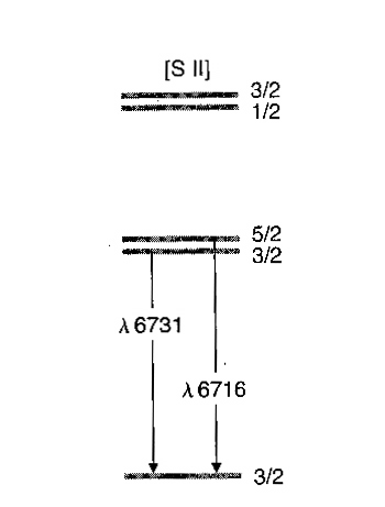
Fig. 1 - Lowest energy levels in singly-ionized sulfur
Astronomers observe spectra of planetary nebulae for many reasons. These spectra contain a wealth of information including the chemical makeup of the gas, its temperature and its density. Such information allows astronomers to connect the properties of planetary nebulae back to the stars that created them, and to understand how planetary nebulae contribute to the chemical enrichment of the Milky Way Galaxy over time. In order to determine the chemical abundances in nebulae, astronomers need to know the temperature of the gas and its density. In this exercise you will learn how and why a particular pair of sulfur emission lines is useful for determining density in planetary nebulae. You will also plot the spectra of several planetary nebulae and estimate their densities using the sulfur lines.
Singly ionized sulfur, S+, has 3 valence electrons. Its electron configuration is 1s22s22p63s23p3. Ions with 3 p electrons have their lowest ground-state energy levels as shown in Fig. 1. Certain electron transitions involve energy levels that are said to be metastable; the resulting emission lines are called "forbidden" lines, which really only means that they are less likely to occur than emission lines from the ordinary kind of transitions. The sulfur emission lines you are studying in this exercise are just such forbidden transitions; in fact, all the upper levels shown are metastable and all transitions among them, as well as to the bottom level, are forbidden.
Ions and electrons in a planetary nebula are always moving and bumping into each other. The energy exchanged in these collisions isn't enough to strip off electrons, but it is enough to kick an electron to a higher energy level within the ground state. For example, a collision could give enough energy to an electron in the bottom level of Fig. 1 for it to jump to one of the higher levels. In fact, the only way that these higher levels can be populated is by collisions; their forbidden nature makes it extremely unlikely for an upward transition to be produced by an absorbed photon.
Notice that the wavelengths of the two lines we are interested are very similar: 6716 and 6731 Angstroms (in the very red part of the visible spectrum). This is because the two originating levels, marked 5/2 and 3/2 in Fig. 1, are so close together in energy. Recall that the wavelength of light and its energy are related by E=hc/λ, where E is energy, h is Planck's constant, c is the speed of light, and λ is wavelength. (Convince yourself that Fig. 1 is correct in assigning the shorter wavelength to the jump from the upper of the two levels.) As a consequence of the closeness in the two energies, just about any collision that could send an electron from the bottom level to the next 3/2 level above it could also send an electron to the nearby 5/2 level, so that both of these levels have about the same chance to be populated by collisions. However, there are two important differences between the 3/2 and the 5/2 levels, and it is precisely these differences that make them useful for density determinations.
One difference is the statistical weight, which is a measure of how many electrons the level can hold. The statistical weights of the 5/2 and 3/2 levels are 6 and 4, respectively - that is, the 5/2 level can hold 6 electrons, while the 3/2 level can accommodate only 4. The other difference is the lifetime: how long, on average, an electron remains in an excited level before spontaneously jumping downward and emitting in this case either a λ6716 or a λ6731 photon. The lifetimes of the 5/2 and 3/2 levels are 3846 seconds (over an hour) and 1136 seconds (almost 20 minutes), respectively. These lifetimes may not seem long to you, but compare them, for example, to an electron in the first excited level in a hydrogen atom which spends an average of only 10-8 seconds before jumping down to the ground state and radiating a photon! That 100 billion-times shorter lifetime means a 100 billion-times higher likelihood of radiating, and that's the difference between an ordinary transition and a forbidden transition.
Just as a collision can excite an electron to a higher energy level, another collision can also knock it back down before it has time to radiate a photon. The much longer lifetime for an electron in a forbidden level means that it is more vulnerable to being collisionally de-excited. The higher the gas density, the more frequent the collisions; that's why we don't see forbidden lines under normal terrestrial conditions - all the electrons in the upper levels are collisionally de-excited before they can radiate.
When the density of the gas is very low, collisions are rare, and most of the electrons that are collisionally excited into upper levels are able to emit a photon as they jump down to the bottom energy level. Under these conditions (below about 100 cm-3), the ratio of the λ6716 line to the λ6731 line is just the ratio of the number of electrons in each level, which is the ratio of the statistical weights, as above, which is 6/4=1.5. The lifetimes don't matter here because even the electrons in the longer-lived 5/2 level have time to radiate. When the gas density is high and collisions are very frequent, the λ6716/λ6731 ratio again approaches a constant value, this time equal to the ratio of the statistical weights divided by the ratio of the lifetimes. The first factor is there for the same reason as in the low density case: the more electrons a level can hold, the more emission there will be. The second factor is needed because now lifetime matters: the less time an electron sticks around in an excited level the more likely it is to be able to radiate before another collision knocks it down, so a short lifetime makes for a stronger line. In the high-density case, above about 10,000 cm-3, the λ6716/λ6731 ratio is about 0.44.
But how are these constant values useful for finding the density in the nebula? They're not. What's useful is this: for densities in between the extremes described above, the observed λ6716/λ6731 intensity ratio depends on the actual density. Think of it this way: as the density increases from a lower limit of about 100 cm-3, the relative lifetimes of the two levels start to come into play as collisions become more frequent. The shorter-lived 3/2 level begins to accrue a slight advantage, and the λ6731 line strengthens relative to the λ6716 line. As the density increases, this trend continues until at around 10,000 cm-3, collisions are so frequent that the shorter lifetime of the 3/2 level confers no further advantage, and the ratio stops increasing. (For comparison, the air you are breathing right now has a density of about 1019 cm-3, or 10 million billion times more than a typical planetary nebula!)
Figure 2 shows how the λ6716/λ6731 ratio behaves as the density changes. Note the region from about 100 cm-3 to 10,000 cm-3 where the ratio drops smoothly from around 1.5 to 0.44. Other ions with similar electron configurations will have their own sets of statistical weights and level lifetimes, and their ratios will be sensitive at different densities.
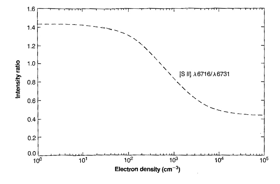
Fig. 2 - Variation of the λ6716/λ6731 ratio as the density changes
The Templates page contains a set of spectra labelled with the wavelengths of emission lines seen in planetary nebulae and identifying the ion producing each emission line. The name of the element is given using the standard chemical symbol from the periodic table (e.g., H=hydrogen, N=nitrogen, Ne=neon, etc.). The ionization state of the element is indicated by a Roman numeral suffix in the following way: neutral=I, singly ionized=II, doubly ionized=III (i.e., ionization state = Roman numeral -1). For example, O III means doubly ionized oxygen, O+2. Conditions in planetary nebulae, as it turns out, are extremely conducive to the production of forbidden lines, and in fact, most of the emission lines you will see in these spectra are forbidden lines, which are denoted by brackets around the ion designation. For example, the designation for forbidden S+ lines is [S II].
All spectra in the database are listed on the Browse page. Clicking on the name of any planetary nebula takes you to the "Spectrum Display" page for that nebula. To expand any region of the graphed spectrum, hold the left mouse button down at one corner of the region you wish to enlarge, drag the mouse to the opposite corner of that region, and then release the mouse button. You can do this repeatedly to keep enlarging. To get back to the full plot, click on the "Zoom Out" radio button under the graph display. The horizontal axis of these graphs is the wavelength in Angstroms, and the vertical axis is the flux (in ergs cm-2 s-1Angstrom-1).
You may find it helpful to print out this page of instructions.
Listed below are five planetary nebulae with different densities. You will examine the spectrum of each nebula and by noting the relative intensities of the [S II] lines, you will be able to estimate the gas density in that nebula.
What is the range of density of these objects?
Consider a typical planetary nebula as a uniformly filled sphere with a radius of 0.1 parsecs (1 parsec=3.1x1018 cm) and a density of 1000 cm-3. Assume that the nebula is pure hydrogen (it isn't, but hydrogen outnumbers helium by a factor of about 10, and all the other elements combined by more than 1000), and calculate how much mass is in the nebula. A hydrogen atom (here just the nucleus, a proton) has a mass of 1.67x10⁻²⁷ kg. Now convert this to solar masses (1 solar mass=1.99x1030 kg). What fraction of the sun's mass does a typical planetary nebula contain?
Click on the image links for these nebulae from the Browse page to see what they really look like. Does the assumption of a uniform sphere seem realistic? In fact, astronomers are trying mightily to design theoretical models of planetary nebulae that reproduce the observed variety of nebular shapes and features.