1	Global Urban Expansion and Commercial Property Stephen Sheppard Williams College Presentations and papers available at http://www.williams.edu/Economics/UrbanGrowth/HomePage.htm
2	Urban Expansion Urban expansion taking place world wide Rich Evolving from transportation choices - “car culture” Failure of planning system? Poor Rural to urban migration Urban bias? Policy challenges Environmental impact from transportation Preservation of open space Pressure for housing and infrastructure provision Policy response Land use planning Public transport subsidies & private transport taxes Rural development Surprisingly few global studies of this global phenomenon Limited data availability
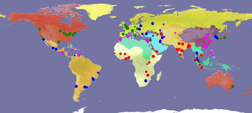
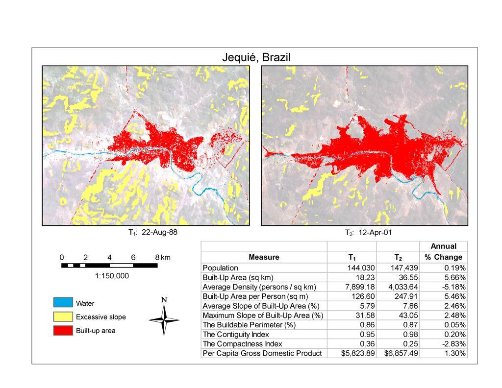
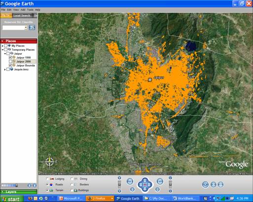
3	Data To address the lack of data, we construct a sample of urban areas The sample is representative of the global urban population in cities with population over 100,000 Random sub-sample of UN Habitat sample Stratified by region, city size and income level
4	Data – a global sample of cities
5	Remote Sensing
6	Measuring Urban Land Use
7	Change in urban land use
8	Display in Google Earth
9	Google Earth Ground View
10	Change in urban land use: Jaipur, India
11	Google Earth view of Jaipur
12
13
14	Modeling urban land use Households: L households Income y Preferences v(c,q) composite good c housing q. Household located at x pays annual transportation costs In equilibrium, household optimization implies: for all locations x Housing q for consumption is produced by a housing production sector
15	Modeling urban land use Housing producers Production function H(N, l) to produce square meters of housing N = capital input, l=land input Constant returns to scale and free entry determines an equilibrium land rent function r(x) and a capital-land ratio (building density) S(x) Land value and building density decline with distance Combining the S(x) with housing demand q(x) provides a solution for the population density D(x,t,y,u) as a function of distance t and utility level u The extent of urban land use is determined by the condition:
16	Modeling urban land use Equilibrium requires: The model provides a solution for the extent of urban land use as a function of Generalize the model to include an export sector and obtain comparative statics with respect to: MP of land in goods production World price of the export good
17	Hypotheses
18	Model estimation We consider three classes of empirical models Linear models of urban land cover “Models 1-3” Linear models of the change in urban land cover “Models 4-6” Log-linear models of urban land cover “Models 7-10” Each approach has different relative merits Linear models – simplicity and sample size Change in urban land use – endogeneity Log linear – interaction and capture of non-linear impact
19	Linear model variables
20	Linear model estimates
21	Models of change in urban land
22	Change in urban land model estimates
23	Log-linear models
24	Log-linear model estimates
25	Hypotheses tested
26	Policy Implications Policies designed to limit urban expansion tend to focus on a few variables Transportation costs and modal choice Combat “car culture” Provide mass transit alternatives Limit road building Rural to urban migration and population growth Enhance economic opportunity in rural areas Residence permits for cities Considerable urban expansion occurs naturally as a result of economic growth Limiting migration could be effective but ... Economic misallocation costs Problems where free mobility considered an important right Importance of the commercial (non-residential) sector Direct impact on land use Indirect via income generation and employment decentralization
27	Implications for Commercial Property What are the implications for non-residential land use? Industrial Export good production Often at urban periphery Office and trade Central and peripheral location These uses compete with residential use Factors that tend to increase urban expansion Promote infill development at central locations Increase non-residential property prices What data are available for analysis?
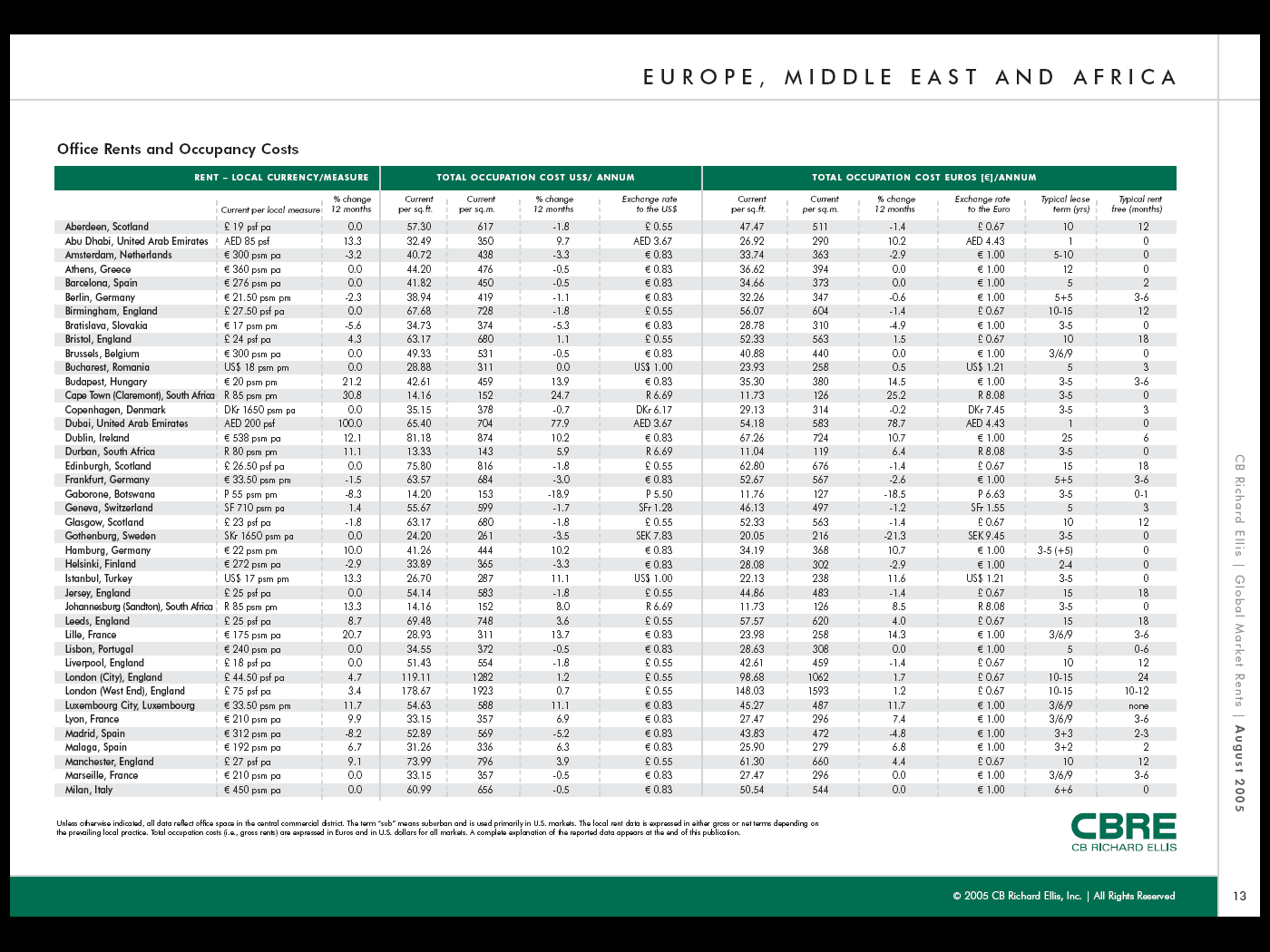
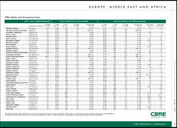
28	Commercial Office Price Data CBRE Global Office Rent Data Data start in 1998 39 of our cities
29	Night Lights Data
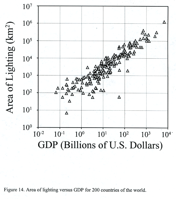
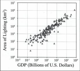
30	Night Lights and Economic Output At the national level Strong relation between lighted area and GDP At the local level Explore potential for disaggregating output to subareas Test this process in US and European cities where employment and output measures are available for subareas
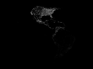
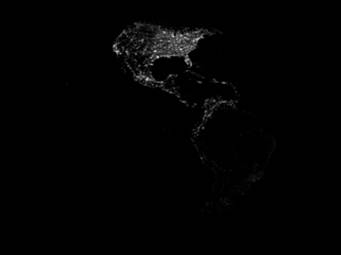
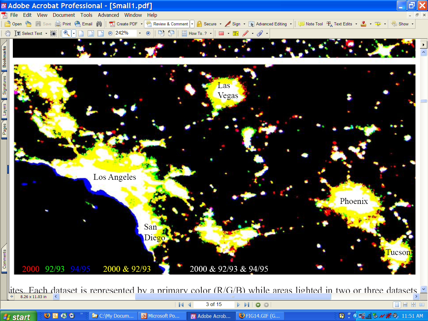
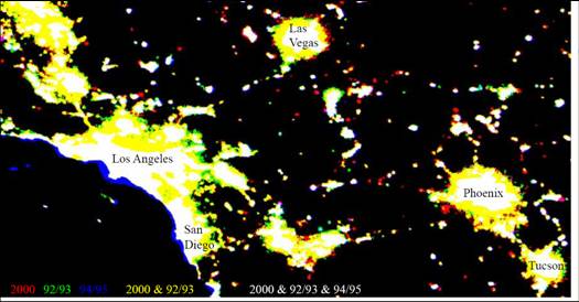
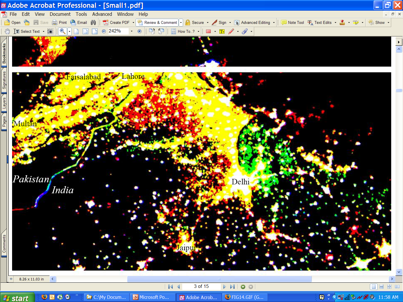
31	Night Lights and Urban Expansion We have light intensity data for three time periods – approximately covering the time period of our land cover measurements
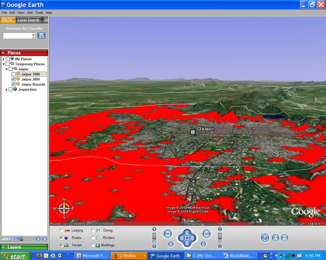
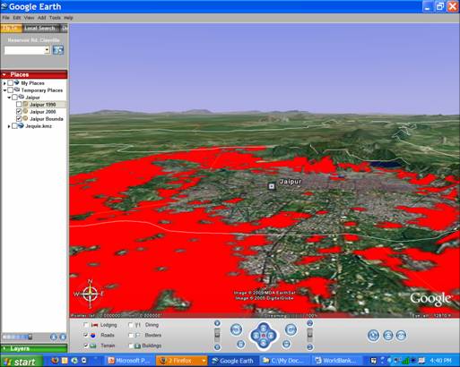
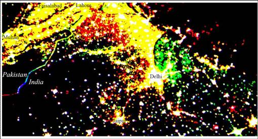
32	Night Lights and Urban Expansion In rapidly changing urban settings, the night light data provide potential for measuring changing land use
33	Potential uses for night light data Limited use for direct identification of urban land use Limited resolving power of data Light diffusion Greater potential as localized index income and employment Use observed illumination to disaggregate national/regional income to local areas Potential when used together with urban land cover measurements Non-residential uses are associated with brighter levels of illumination As a localized index of commercial land use, consider:
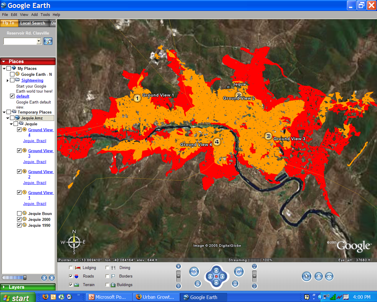
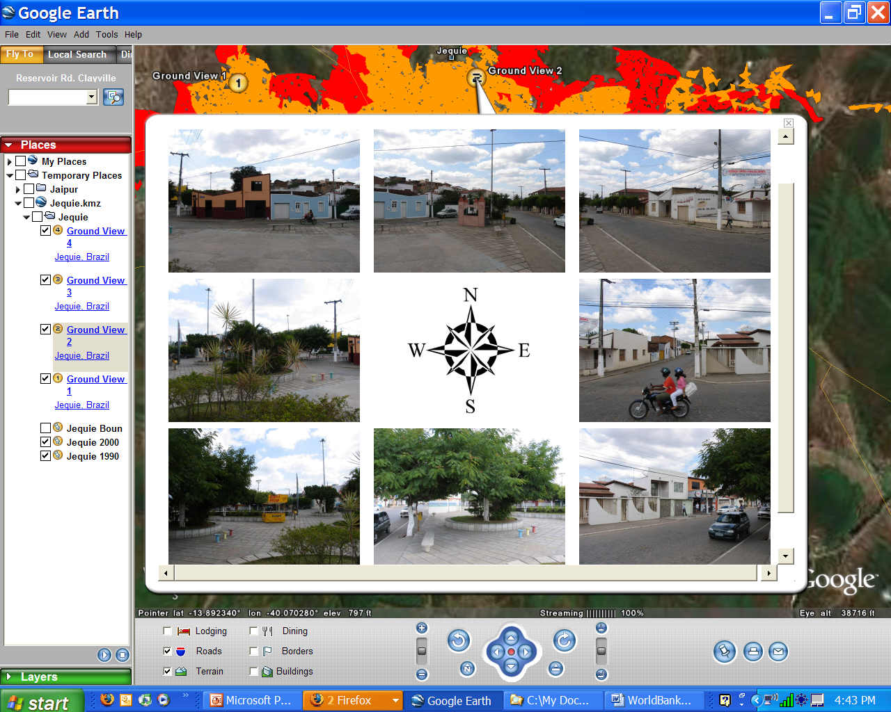
34	Data and econometric chores Many issues to address going forward Endogeneity issues Transport costs Income Links to global economy Effectiveness of planning policies Availability of housing finance In progress Field research to collect data Evaluation of classification accuracy Modeling at micro-scale – transition from non-urban to urban state Interaction with other local development
35	Hypotheses Maintained hypothesis: that non-residential urban land use is more intensively lit than residential (or detected as such) Increased linkage to global economy increases industrial land use Increased ratio Increased industrial land use increases employment suburbanization Increased sensitivity of urban expansion to income Decreased sensitivity of urban expansion to transport (fuel) costs Factors promoting urban expansion will increase commercial property rents Explore potential for identification of separate impacts of income and automobile transport