Additional comments related to material from the class. If anyone wants to convert this to a blog, let me know. These additional remarks are for your enjoyment, and will not be on homeworks or exams. These are just meant to suggest additional topics worth considering, and I am happy to discuss any of these further.

• Friday, May 15. Today's question on the universality of spacings / results is one of the central ones in modern mathematics and science. What I've seen over the past few years / decades is that this universality is frequently due to the fact that the answer depends only on the first two moments, and the higher moments affect the rate of convergence. We saw this a bit when we looked at the zeros of Dirichlet L-functions and when we looked at the density of states in random matrix theory (only the first and second moments mattered there). Today we discussed the proof of the Central Limit Theorem. We saw the density for the sum of two independent variables X1 and X2 with densities f1 and f2 is given by Prob(X1 + X2 = x) = Int_{-oo to oo} f1(t) f2(x - t) dt; this is called the convolution of two functions, and is denoted (f1 * f2)(x). The proof uses the fact that the Fourier Transform of a convolution is the product of the Fourier transforms and that lim_{n --> oo} (1 + x/n)^n = exp(x). The reason we did not give a full proof is that we needed to use the inverse Fourier transform, and we never showed that the inverse Fourier transform of certain nice functions is unique. For details see sections 11.4.3 and 11.5 in our book.

• Wednesday, May 13. Today we analyzed the first sum (the (log p / sqrt(p) log m) chi(p) ... term) in the explicit formula for the family of Dirichlet L-functions (arising from chi: (Z/mZ)* to Complex Numbers of Absolute Value 1). We saw that if the Fourier transform of our test function h has support in (-sigma, sigma) with sigma < 2 then these terms do not contribute as m --> oo. The two inputs for this were the following; (1) a formula for summing chi(n) over all chi in our family (this was -1 if n wasn't equivalent to 1 mod m and m-1-1 if n was); (2) trivially estimating the two resulting sums, one over all primes and one over primes congruent to 1 modulo m. Almost surely one can do better. We attacked this problem the same way we've attacked numerous others: put in absolute values and take worst case scenarios every single time. Inputting more number theory should lead to us getting better results. There are numerous papers which have estimates that are similar to what we need (ie, estimates for error terms in the distribution of primes in arithmetic progression), but sadly none of these have provable results which help (they do have conjectures which help). If you're interested, let me know and I'll send you some papers to read. A good first paper to get some familiarity with the subject is Montgomery's Primes in Arithmetic Progression.

• Monday, May 11. As always, see Chapters 3 and 18 of our book for more information about Dirichlet Characters and Dirichlet L-funcions. Their main applications are in proving Dirichlet's Theorem of Primes in Arithmetic Progression and other similar results. We showed today how to modify the explicit formula for the Riemann zeta function to obtain one for Dirichlet L-functions. We assumed the Generalized Riemann Hypothesis, which allows us to write the non-trivial zeros of L(s,chi) as 1/2 + i gamma_rho, where gamma_rho is a real number. This led to an explicit formula (see Chapter 18 for the details) relating sum_rho h(gamma_rho * log m) to sum_p log p h^(log p / log m) / sqrt(p).  We discussed in detail why we have a function h on the zeros side and its Fourier transform h^ on the prime side. In Wednesday's class we'll analyze these sums (if you want to read ahead and see all the details, the preprint is available here). This falls out naturally from the logarithmic derivative and choosing our test function to be nice when Re(s) = 1/2. Specifically, we're integrating (1/2 pi i) Int_{Re(s) = 1+epsilon} phi(s) ds / n^s, where phi(s) = h( (s - 1/2) / i ) for some nice function h. When we shift contours to Re(s) = 1/2, we have s = 1/2 + it so ds = i dt and the integral becomes (1 / 2 pi) Int_{t = -oo to oo} h(t) dt / n^{1/2 + it} = (1 / 2 pi) (1 / sqrt(n)) |int_{t = -oo to oo} h(t) exp(-2 pi i (log n / 2 pi) t) dt, and this integral is just h^(log n / 2pi). We also talked a bit about how to write down formulas for each Dirichlet character, using the fact that (Z/mZ)* is a cyclic group for m prime. We saw each group is generated by some element g, so a typical element x = g^k for some k. It therefore suffices to define the Dirichlet character at the generator. As these characters map (Z/mZ)* to complex numbers of absolute value 1 and are group homomorphisms, we have |chi(g)| = 1, chi(g^{m-1}) = chi(g)^{m-1} = 1 and chi(1) = 1, implying that the characters are the same as the functions    f(g) = exp(2 pi i ell / (m-1)) for ell in {0,1,...,m-2}. If ell = 0 we basically recover the Riemann zeta function when we look at Sum_n chi(n) / n^s; for other n, however, we get very different functions. These functions are significantly easier to extend past Re(s) = 1 because of the cancellation in sums of chi(n). In fact, if ell is not zero, then the associated character chi satisfies Sum_{n=0 to m-2} chi(n) = 0. This and partial summation allow us to extend Sum_n chi(n) / n^s from Re(s) > 1 to Re(s) > 0. We briefly mentioned random harmonic series: Sum_n omega(n) / n where omega(n) = 1 with probability 1/2 and -1 with probability 1/2. Schmuland has a fascinating paper on the properties of these sequences (try here if that link doesn't work).

• Friday, May 8. The Riemann zeta function is the first of many such functions we can study. The generalizations are called L-functions, and for us are of the form L(s,f) = Sum_n a_n(f) / n^s = Prod_p L_p(s,f)^{-1} where L_p(s,f) is a polynomial of degree d in p^{-s}. Two of the most important are Dirichlet L-functions (which has applications to primes in arithmetic progression) and Elliptic Cuve L-functions (which has applications to understanding the size of the group of rational solutions of the elliptic curve -- see the Birch and Swinnerton-Dyer conjecture for more information). Dirichlet characters are sometimes covered in a group theory or abstract algebra course. If you want more details, see Chapter 3 of our book (from Section 3.3.2 to 3.3.6). Elliptic curves are discussed in Section 4.2.We initially used some knowledge of the zeros of the Riemann zeta function to deduce information about the primes. Amazingly, if we look at families of L-functions we can convert knowledge of sums over the family of the a_n(f) to information about the zeros of the associated L-functions. We saw how we have great formulas for summing Dirichlet characters; similar formulas exist for other families as well. For details in the case of Dirichlet L-functions, see Chapter 18 of our book. Note the amazing similarity between random matrix theory. We have three ingredients to understand the zeros. (1) Determine the correct scale to study the zeros (this actually falls out from the functional equation). (2) Derive a formula relating sums over the zeros to a related sum over the prime coefficients. This is the analogue of the Eigenvalue Trace Lemma, Tr(A^k) = Sum lambda_i(A)^k. The reason this formula was so useful is that while we want to understand the eigenvalues of our random matrices, it is the matrix elements that we choose. Thus, this formula allows us to pass from knowledge of the matrix elements to knowledge of the zeros. These are known as Explicit Formulas. (3) The Eigenvalue Trace Lemma and the Explicit formula would be useless, however, if we were unable to actually execute the sums. Our theory thus requires some kind of averaging formula. For random matrix theory, this was the integrals of Tr(A^k) P(A) dA; we could compute these as Tr(A^k) is a polynomial in the matrix elements, and then we used combinatorics and probability theory. Sadly, we do not have great averaging formulas in number theory, and this is why the results there are significantly worse.

• Wednesday, May 6. The complex analytic proof of the Prime Number Theorem uses several key facts. We need the functional equation of the Riemann zeta function (which follows from Poisson summation and properties of the Gamma function), the Euler product (namely that zeta(s) is a product over primes), and one important fact that no one questioned in class: what if the Riemann zeta function has a zero on the line Re(s) = 1! If this happened, then the main term of x from integrating zeta'(s)/zeta(s) * x^s/s arising from the pole of zeta(s) at s=1 would be cancelled by the contribution from this zero! Thus it is essential that there be no zero of zeta(s) on Re(s) = 1.  There are many proofs of this result. My favorite proof is based on a wonderful trig identity: 3 + 4 cos(x) + cos(2x) = 2 (1 - cos(x))^2 >= 0 (many people have said that w^2 >= 0 for real w is the most important inequality in mathematics). If people are interested I'm happy to give this proof in class next week (or see Exercise 3.2.19 in our textbook; this would make a terrific aside if anyone is still looking for a problem). There is an elementary proof of the prime number theorem (ie, one without complex analysis). For those interested in history and some controversy, see this article by Goldfeld for a terrific analysis of the history of the discovery of the elementary proof of the prime number theorem and the priority dispute it created in the mathematics community. We mentioned Riemann computed zeros of zeta(s) but didn't mention his achievement; the method only came to light about 70 years later when Siegel was looking at Riemann's papers. Click here for more on the Riemann-Siegel formula for computing zeros of zeta(s). Finally, terrific advice given to all young mathematicians (and this advice applies to many fields) is to read the greats. In particular, you should read Riemann's original paper. In case your mathematical German is poor, you can click here for the English translation of Riemann's paper. The key passage is on page 4 of the paper:
  • One now finds indeed approximately this number of real roots within these limits, and it is very probable that all roots are real. Certainly one would wish for a stricter proof here; I have meanwhile temporarily put aside the search for this after some fleeting futile attempts, as it appears unnecessary for the next objective of my investigation.
     

• Monday, May 4. Today's lecture highlights the connections between complex analysis and number theory. The key relationship is the logarithmic derivative of the Riemann zeta function is a sum of primes. There are two expressions for the Riemann zeta function when Re(s) > 1, one as a sum over integers and one as a product over primes. While typically the sum is easier to work with, it is the product expression that is more useful here (not surprisingly as we are interested in properties of primes). Whenever we see a product we want to take a logarithm, and thus it is natural to take the logarithm of the product expansion. This product expansion is called the Euler Product, and is one of the most useful properties of the Riemann zeta function. We then showed (or rather sketched the argument -- we'll provide more details on Wednesday) by contour integration that Sum_{p <= x} log p + nice(x) = x - sum_{rho a zero of zeta(s)} x^rho / rho. This is the Explicit Formula of the Riemann Zeta Function (see Chapter 18 for more details), and shows how we can pass from knowledge of the zeros to knowledge of the primes. The Riemann Hypothesis asserts that all the non-trivial zeros have real part equal to 1/2; this basically implies that the error term in the Prime Number Theorem is of size x^{1/2 + epsilon} for any epsilon > 0. We will explore in greater detail connections between fine properties of these zeros and properties of the primes specifically and other number theoretic functions in general. For example, the class number is extremely important in additive number theory, and the best unconditional bounds on its size are significantly less than we expect is true. It is now believed that the spacing statistics of the Riemann zeta zeros agrees with that of eigenvalues of the Gaussian Unitary Ensemble (an important class of random matrices); if true (or even if we could just prove some weaker results towards this conjectured agreement), we end up with bounds for the class number of the expected order of magnitude. For details, see the paper Spacing of Zeros of Hecke L-Functions and the Class Number Problem by Conrey and Iwaniec. Other applications of fine properties of the distribution of the zeros, the Grand Simplicity Hypothesis, are important in analyzing Chebyshev's bias; see Chebyshev's Bias by Rubinstein and Sarnak.

• Wednesday, April 29. To see the connection between zeros of the Riemann zeta function and the distribution of primes requires some results from complex analysis. The main input we will need is that integrals along circles (or more generally nice curves) of the logarithmic derivative of a nice function is just the order of the zero or pole at the center of the circle. In other words, if we have a Taylor expansion f(z) = a_k z^k + ... (where k is the first non-zero term; thus a_k is not zero and if k > 0 we say the function has a zero of order k at the origin, while if k < 0 we say the function has a pole of order k). The Residue theorem then gives: (1 / 2 pi i) Integral_{|z| = r} f'(z)/f(z) dz = k. Note that if the function doesn't have a zero or pole at the origin then this integral is zero (for r sufficiently small). More generally, if g(z) is a nice function (1 / 2 pi i) Integral_{|z| = r}g(z) f'(z)/f(z) dz = k g(0). We will use a further generalization of this on Monday to relate the zeros of the Riemann zeta function to counting the number of primes at most x. For more details on the complex analysis we are using, see Cauchy-Riemann equations, Cauchy-Goursat Theorem, Residue Theorem, Green's Theorem.
The key takeaways from today's class are: (1) we can convert certain types of integrals to finding the a_{-1} coefficient in a Taylor expansion (and this is good as algebra is easier than integration); (2) integrating the logarithmic derivative is useful as the answer is related to the zeros and poles of the function.


• Monday, April 27. There are many proofs of the functional equation of the Riemann zeta function; the proof we gave is `secretly' relating the Riemann zeta function to the Mellin transform (which is basically the Fourier transform after a change of variables) of the theta function. A crucial input was the Gamma function, which arises throughout mathematics, statistics, science, .... Functional equations are extremely important, as they allow us to work with useful functions that are initially only defined in one region in larger regions. The functional equation of the Riemann zeta function or the Gamma function (or the geometric series) are just a few instances. It is worth pondering what allows us to find a functional equation. For the Gamma function, it was integrating by parts in the integral defining the Gamma function; for the theta function, it was Poisson summation. Finally, it is worth noting that we have seen yet again examples of how problems can be converted to integrals. In this case, the Riemann zeta function initially was only defined for Re(s) > 1; however, we then rewrote it as an integral from x = 0 to oo involving the omega function (which also made sense only for Re(s) > 1),  but then we rewrote that as two integrals from x = 1 to oo involving the omega function, and these integrals exist for all s. We are fortunate in finding an integral expression which we can work with. It should hopefully seem `natural' (at least in hindsight) in passing from the omega function to the theta function (omega is a sum over n > 0, theta is a sum over all n and thus there is a chance Poisson summation could be useful).

• Friday, April 24. Many of the Riemann zeta function's properties are related to viewing it as a function of a complex variable s. As such, it is not surprising that we need some results from Complex Analysis for our studies. The main result we are heading towards is the Cauchy Residue Theorem. The most important fact is that if f(x) = Sum_{n = -N to oo} a_n z^n, then (1 / 2pi i) Int_{|z| = r} f(z)dz = a_{-1}. The reason this is such a spectacular formula is that it reduces integration (hard) to finding ONE Taylor coefficient (ie, algebra, ie easy). Finally, below are the three arxiv posts I mentioned related to either topics we've just studied or are about to (note: the arxiv is a wonderful site, but nothing on it is refereed; many professional mathematicians check the arxiv every day and skim the titles and abstracts of all posts; many more do this for their speciality)
  • The ternary Goldbach problem with arithmetic weights attached to two of its variables (Tolev)
  • Expansion and improvement of sieve and applications in Goldbach's problem (Ren)
  • Eigenvalue density, Li's positivity, and the critical strip (He, Jejjala, Minic)

• Wednesday, April 22. Creating prime deserts efficiently is an interesting challenge (one can try to prove the existence of gaps or one can try and construct explicitly such a gap); see the wikipedia entry for a description of known results. Note that the (k+1)! method Bryan mentioned means we need to look at numbers of size 10^5768 to find a gap of size 2009;  The correct notation for Ralph's prime factorial is #, called the primorial (see the link for a nice summary of how it grows relative to the factorial function.); using the primorial function we see it suffices to `merely' go up to about 10^845 (hey, it's large but it's better than where our results kick in for the sum of three primes, and it does beat using Chebyshev, I think). Trying to find good upper and lower bounds for phi(q), Euler's totient function, is but one of many problems concerning the standard arithmetic functions. One is often interested in average values, standard deviations, et cetera of such functions. A great source for such material is Hardy and Wright's classic An Introduction to the Theory of Numbers (you should also read Hardy's A Mathematician's Apology for a description of one person's reasons for doing math). Other functions that are fascinating to study (as q varies) is the divisor function, the number of distinct prime factors, .... Finally, partial summation is one of the most frequently used tools in number theory and analysis, for two reasons: (1) it allows us to pass from a sum we know to one we want to know; (2) it replaces sums with integrals, and we have more closed form expressions for integrals. We used partial summation today to prove that the sum of the reciprocals of the primes at most x grows like log log x, which we then used to prove phi(q) > C q / log log q. This is but one of many applications of partial summation (and but one of many proofs that the sum of the reciprocals of the primes diverge).

• Monday, April 20. RSA encryption is just one of many encryption schemes based on number theory. The pirate example we mentioned (transmitting a secret from island to island) is an example of key exchange; one popular method is the Diffie-Hellman key exchange (it was quite surprising to some that there was a way for two people to agree upon a secret knowable only to them without meeting in person to exchange the secret). The key ingredient in proving RSA works is Fermat's little Theorem. Thus the key ingredients in our analysis are some of the standard functions of number theory (such as the Euler totient function), efficient computations algorithms (such as fast exponentiation and the Euclidean algorithm, both of which are described in detail in Chapter 1 of our book), and of course the need to have a fast way to determine if a number is prime. There have long been known good, efficient methods to check primality, but these either were probabilistic or depended on the Riemann hypothesis; a few years ago Agrawal, Kayal and Saxena gave an explicit, deterministic polynomial time algorithm, Primes in P. We also briefly discussed other efficient algorithms for multiplying matrices. The Strassen algorithm (see also the Mathworld entry here, which I think is a bit more readable) multiples two NxN matrices A and B in about N^(log_2 7) multiplications; the reason for this savings is that they can multiply two 2x2 matrices with seven and not 8 multiplications (3 = log_2 8). The best known algorithm is the Coopersmith-Winograd algorithm, which is of the order of N^2.376 multiplications. See also this paper for some comparison analysis, or email me if you want to see some of these papers. Some important facts. (1) The Strassen algorithm has some issues with numerical stability. (2) One can ask similar questions about one dimension matrices, ie, how many bit operations does it take to multiply two N digit numbers. It can be done in less than N^2 bit operations (again, very surprising!). One way to do this is with the Karatsuba algorithm (see also the Mathworld entry for the Karatsuba algorithm). Finally, we ended with a discussion of the group structure of elliptic curves, which replaces the group (Z/pqZ)* with a more complicated group and thus open up another possibility for encryption. In both systems the difficulty in cracking the code comes from having to solve the discrete log problem.

• Friday, April 15. The main accomplishment of today was three false attempts at trying to prove that an even number can be written as the sum of two primes (also known as the Binary Goldbach problem). Though we didn't succeed, it is illuminating to see what approaches are `natural' and why they may or may not work. In particular, approximating the integral of a non-negative function through the Cauchy-Schwartz inequality does frequently work in many problems.

• Wednesday, April 15. Today we emphasized heuristics to see if the Circle Method has a chance of working. One of the HW problems gives lower bounds for how many k^th powers are needed so that all integers are a sum of at most that many k^th powers; surprisingly, this lower bound turns out to be the correct answer for many problems (ie, we need at least this many terms to suffice for some integers, and in fact this will suffice for all integers); see the article on Wikipedia for more details. Before doing long calculations it is worthwhile to try some quick rough estimates to get a sense of whether or not the method has a chance of success.

• Monday, April 13. The Mathematica code to investigate problem 1 on the midterm is available here. Note that most of the bad n's are multiples of 99; it's an interesting question (at least to me!) as to what the best m is for a given n (recall the problem is: given any integer n > 1 find an integer m such that nm only has 0s and 1s in its base 10 expansion, and if possible find the smallest m for a given n). We can give constructive solutions, but for the most part the numerical investigations show these constructive solutions are far larger than needed. For the second problem (on approximating irrationals by rationals of given forms), the first part asks about how small |alpha - n/q| can be when q is prime. We showed (trivially and with great effort!) that we can do |alpha - n/q| < 1/q, but one can do better. See the comments from Monday, March 16th, especially the article on Wikipedia for a general description or the paper by Baker, Harman and Pintz for the details.    Finally, here is a fascinating clip of a great speaker talking about the importance of asking the right question.

• Friday, April 10. Looking for obstructions to Diophantine equations is a great way to start to investigate whether or not there is a solution. In particular, if an equation f(x1, ..., xn) = 0 is to be solvable in the integers two things must hold: (1) it must have a solution with each xi real; (2) it must have a solution modulo p for each prime, ie, f(x1,...,xn) = 0 mod p. While we can use this to prove certain equations don't have solutions (x1^2 + x2^2 + 2009 = 0 has no real solution, and 2x1 + 2x2 - 2009 = 0 has no solution modulo 2), it is not the case that if these two conditions hold than the equation has an integer solution. The classic example is 3x^3 + 4x^3 + 5x^3 = 0 (due to Selmer). The hope is that somehow (often using the Chinese Remainder Theorem) we can piece together the local solutions for each prime p to form a global solution to the original problem. This is known as the Hasse Principle (works well for quadratics, but as Selmer's example shows it does not work in general). We also discussed the Philosophy of Square Root Cancellation (ie, the Central Limit Theorem) (see pages 213 to 215 of our book for a proof in the special case of tossing a fair coin). See also this blog entry by E. Kowalski. If you want to numerically explore and see the square-root cancellation in practice, you can go to the following applet on the web. Finally, there was a nice post on the arxiv recently by Boklan and Elkies: Every multiple of 4 except 212, 364, 420, and 428
  is the sum of seven cubes.

• Wednesday, April 8. The numerics of the main term of the Hardly-Littlewood conjectures show a phenomenal agreement with numerics (for predicting twin primes at most x; similar agreement is seen in other problems); unfortunately, in general proving the error term is small is beyond all current techniques. See the nice blog post by Terry Tao for more on randomness in primes and predictions. The current record for writing large odd numbers as the sum of three primes is that any odd number at least 10^1346 is the sum of at most three primes (this number is far beyond the range of anything we can investigate on the computer). The key ingredient in our investigations is to use generating functions; the difficulty is finding such functions whose coefficients encode the information we want while being tractable enough to work with. One enormous advantage of the modern formulation of the Circle Method to the original is that we just use finite series; this avoids many convergence issues and simplifies the analysis.

• Monday, April 6. We discussed two of the main ingredients in the Circle Method: (1) writing expressions as Main Term + Error with good control on the error, and (2) proving something happens at least once by showing it happens many times. We discussed prime races (see also here), and how misleading the data can be. Instead of looking at pi_{3,4}(x) - pi_{1,4}(x) we could look at Li(x) - pi(x); this was also observed to be positive as far as people could see, but it turns out that they flip infinitely often as to which is larger. This was shown by Littlewood, but it was not known how far one must go to see pi(x) > Li(x). His student Skewes showed it suffices to go up to 10^(10^34) if the Riemann hypothesis is true, or 10^(10^(10^963)) otherwise (as large as these numbers are, they are dwarfed by Graham's number). We 'believe' it's around 10^316 where pi(x) beats Li(x) for the first time (note this is well beyond what we can investigate on the computer!). The proof involves the Grand Simplicity Hypothesis (that the imaginary parts of the non-trivial zeros of Dirichlet L-functions are linearly independent over the rationals); this is used to show that (n gamma_1, ..., n gamma_k) mod 1 is equidistributed in [0,1]^k where the gamma_j are the imaginary parts of these zeros. Note that this is Kronecker's theorem (which we discussed in one of the homework problems); it's amazing how this result surfaces throughout mathematics. We'll continue on Wednesday with the Circle Method applied to certain Diophantine Problems; if anyone is interested in looking at the Catalan Conjecture (now a theorem) and its relation to no product of four consecutive integers is a square, let me know. We ended with a brief discussion on how instead of looking at A+A+...+A we could look at A-A; for example, if A = P (the set of primes), we know 2 is in P-P. What is nice about the Circle Method is the way it proves something is in a set like A+A+...+A or A-A is to count how MANY times it is in. Thus, the Circle Method will give heuristics as to how many times 2 occurs in P(N) - P(N), where P(N) is the set of primes at most N. This leads to the Hardy-Littlewood heuristics for the number of twin primes. In our book we study how many Germain primes there are, primes p such that (p-1)/2 is also prime. These primes have applications in cryptography (in proving that it is possible to do primality testing in polynomial time (see also here) -- if there are as many Germain primes as the Circle Method predicts, certain primality tests run faster) and in Fermat's Last Theorem (if  x^p + y^p = z^p and p is a Germain prime then p|xyz).

• Friday, March 20. TBD: We'll almost surely talk about Poisson Summation and its applications. One fun application is to proving the iterates of the 3x+1 map satisfy Benford's law. The 3x+1 is just one of many fascinating sequences to study; another great one is Conway's See and Say (or Look and Say) sequence: 1, 11, 21, 1211, 111221, .... There are numerous fascinating properties of these sequences; one of my favorites is the Cosmological Theorem and the interpretation of terms in the sequence in terms of elements in the periodic table! There were several proofs of this wonderful theorem; unfortunately they were all `lost'. Since then new ones have appeared; see the write-up here for a proof. The first author of the paper is Shalosh B. Ekhad; if you've never met `Professor Ekhad' I strongly urge you to click on the link and take a look at the `Professor' (who is the first author of the paper!).

• Wednesday, March 18. Poisson Summation is one of the standard tools of analytic number theory, allowing us to frequently convert long, slowly decaying sums to short, rapidly decaying sums, so that just a few terms suffice to get a good estimate. One nice application is to counting the number of lattice points with integer coordinates inside a circle (also called the Gauss circle problem). If you consider points with integer coordinates, you would expect approximately pi R^2 such points to be in a circle of radius R; what is the error? A little inspection shows that the error shouldn't be much worse than the perimeter, so the answer might be pi R^2 with an error of at most something like 2 pi R (Gauss proved an error of at most 2 sqrt(2) pi R). The current record is by Hooley, who shows that the error is at most C R^theta, where theta <= .6298.... We also looked at the Fourier Transform and interesting functions that satisfy a lot of nice conditions but not every property we'd like. See for example the function f on page 270 (or better yet modify this to be infinitely differentiable and it and its first five powers are integrable).

• Monday, March 16. Today we chatted about spacings between primes, and consequences. We discussed Chebyshev's theorem (we prove a version on page 40 of our textbook) that for all x sufficiently large, there are numbers A and B with 0 < A < 1 < B < oo such that the number of primes pi(x) satisfies Ax/ln(x) <= pi(x) <= Bx/ln(x); we used this to prove Bertrand's postulate that there is always a prime between n and 2n. We then discussed the Principle of Inclusion - Exclusion (see pages 18 and 44) and used this to prove that if we rearrange n people, as n --> oo the probability no one is back where they started tends to 1/e (this is known as a derangement). Using inclusion / exclusion, Brun was able to prove the sum of the reciprocals of twin primes converge. If we set pi_2(x) to be the number of twin primes at most x, he showed pi_2(x) < C x (log log x)^2 / (log x)^2; I used it was at most C x / (log x)^{3/2} in class, a MUCH weaker result. Our proof in class is typical of many results in number theory -- be as crude as possible as long as possible in your estimations; if you don't get your result, then refine your estimates as needed. We did numerous 'worst case' approximation and still won. Now, if we asked a harder question (estimate the RATE of convergence), then we of course couldn't be so crude. Many of our arguments used dyadic interval decompositions (as does the proof of Chebyshev given in our book). For the original question as to what is the best known result about spacings between primes? Well, this depends on what one assumes. We believe there is always a prime between n^2 and (n+1)^2; when I started grad school I believe the best unconditional result was there is a prime between x and x + c x^{7/12}, which has been improved to a prime between x and x + x^.525 (see the article on Wikipedia for a general description, or the paper by Baker, Harman and Pintz for the details.) In particular, we've known for awhile that there is a prime between n^3 and (n+1)^3 (which is basically between x and x + C x^{2/3}). One of the ways we proved results such as these is to show that there are MANY primes in the region, and thus there is at least one. This is another common number theory technique, and we'll see it again in the Circle Method. (Another occurrence is proving there is at least one prime congruent to a mod b if a and b are relatively prime; the only way we can do this in general is to prove there are INFINITELY many such primes, and in fact that they occur in the right proportion; this is Dirichlet's Theorem on Primes in Arithmetic Progression, included in Chapter 3 of our book.) We discussed how there can't be a prime triple of the form p, p+2 and p+4 other than 3, 5, 7; this leads to the question of just which arithmetic progressions are possible. The largest to date might be an arithmetic progression of length 25; Green and Tao proved that there are arbitrarily long arithmetic progression (sadly it's an existence theorem, with nothing said about actually finding one!).

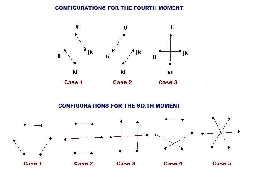
• Friday, March 13. In discussing the various fourth, sixth and general moment calculations, we saw two key points. The first is that there can't be a contribution to the main term unless we are matched in pairs; however, being matched in pairs is only a necessary but not a sufficient condition for a main term contribution. For all real symmetric matrices, it seems the contribution to the main term of the even moments occurs only when things are in a generalized matched pairing with neighbors. This means that we can remove the paired edges one at a time. For example, consider the matchings in the fourth and sixth moments below. The first two cases in the fourth moment contribute, but the third doesn't. When you look at the number of free indices, it's three in cases 1 and 2 but only one or two in case 3. Similarly, in the sixth moment only cases 1 and 2 contribute. These have everything in a generalized match with a neighbor. While this is clear for case 1 of the sixth moment, it isn't immediately clear for case 2. What happens is that if two neighbors are matched, we can 'remove' that matching from our graph and look at what remains, and we have one free variable as we remove. For example, we first remove the top and then the bottom matching in case 2, and what remains is just a neighbor matching. Why does this work? Say a_{no} is matched with a_{op}; thus our string looks like a_{mn}, a_{no}, a_{op}, a_{pq}. As a_{no} and a_{op} are matched, 'o' is a free variable, and n=p. We can then lift this matching out, and this collapses to a_{mn}, a_{n,q}. Thus it reduces to a smaller graph. In general, the combinatorics depend crucially on the structure of the real symmetric matrices under consideration. We get very different combinatorics for d-regular graphs. Another fun example is Toeplitz matrices (these matrices have applications in computer science, and connections with Fourier series; they are constant along diagonals and thus have far fewer degrees of freedom than a general real symmetric matrix). The combinatorics are very different; for real symmetric Toeplitz matrices case 3 of the fourth moment now contributes. This isn't too surprising, as we now have many ways for two indices to be the same; we don't just need say {i,j} = {m,n}, but only that they be on the same diagonal (or on reflected diagonals, ie, |i-j| = |m-n|). For real symmetric Toeplitz matrices (the link is to my paper with students on the subject), however, there are still some obstructions in the combinatorics. While there are (2m-1)!! matchings in pairs, not all of the matchings contribute fully; if they did, the density of states would be a Gaussian, as (2m-1)!! is the 2m^th moment of the Gaussian. The fourth moment of these matrices is 2 2/3, not 3 (we have freedom to adjust to make the first two moments be 0 and 1, but after that the later moments show the true shape of the distribution). This is seen in that we have equations such as i = j + k - l with all indices in {1,...,N}, but if j,k > 2N/3 and l < N/3 then there is no valid i; these Diophantine obstructions cause the moment to be less than the Gaussian. If we add the condition that the first row be a palindrome, then these obstructions vanish, and the density of states for Real Symmetric Palindromic Toeplitz matrices (the link is to my paper with students on the subject) is the Gaussian.
  

• Wednesday, March 11. Today we finished the proof of the odd moments for Wigner's Semicircle Law. We were fortunate that we don't need to determine all the possible matchings; all we needed to know was that, for fixed k = 2m+1, the number of matchings where everything is matched in at least a pair is independent of N. The combinatorics for the even moments are more delicate, as these do contribute and we will need to know exactly how many there are. This leads to the Catalan numbers. Though it isn't needed, it's an interesting question to ask how many solutions there are to r_1 + r_2 + ... + r_n = 2m+1 where each r_i >= 2 and n can range from 1 to m. This is an example of a Diophantine equation, at least when n is fixed. Diophantine equations arise in many problems, and lots of people spend their life looking for integer solutions to equations (or systems of equations) involving polynomials with integer coefficients. There is a well-developed theory to these problems, and it is surprisingly easy (once you look at things the right way, which is how much of combinatorics is!) to incorporate conditions such as each r_i >= 2; allowing n to be free is harder. A good extra credit problem is to determine the number of such matchings.

• Friday, March 6. We analyzed the third moment for the density of eigenvalues of real symmetric matrices. For the third moment the assumption that the density p(x) is even helped but not enormously so; for the higher odd moments it initially looks to be quite useful (as it allows us to avoid some messy combinatorics). We'll see on Wednesday that the combinatorics can be bypassed for the odd moments by a simple counting argument (namely, that as long as the density p(x) has finite moments, there aren't enough matchings to contribute in the limit). This is violently false for the even moments. There we will have to do some subtle combinatorics (in fact, the differences in the density of states between different families of real symmetric matrices is due to the differences in combinatorics that arise). We'll see the answer is related to the Catalan numbers. We also discussed the `cookie problem' (see chapter 1 of our textbook). This is actually the k=1version of Waring's problem; unfortunately the combinatorial argument to solve the k=1 case does not generalize to the higher cases. There are many techniques to analyze combinatorial problems; one of my favorites is matching coefficients (see my handout from my mathematical statistics course from my Brown days).

• Wednesday, March 4. We saw how the number of degrees of freedom in our random matrix ensemble greatly affects the density of eigenvalues, but surprisingly doesn't seem to affect the spacings between normalized eigenvalues. In some sense, these spacings between events are universal (and there is just a rescaling going on). One reason I love number theory / random matrix theory so much is the connections between behavior here and in other systems. A great question from class today was why we only looked at the spacings between the eigenvalues in the middle of the semi-circle (this is called the 'bulk' of the spectrum) and not near 1 or -1 (called, not surprisingly, the 'edge' of the spectrum). The behavior of the largest eigenvalue is well understood, and given by a Tracy-Widom distribution (for real symmetric matrices, a TW distribution with beta = 2). The TW distribution occurs in many other interesting places, including the length of the longest increasing subsequence.

• Monday, March 2. Today we reviewed the probability we'll need, moments and the method of moments (note the Wikipedia entry specifically mentions Wigner's Semi-Circle Law, and no, I wasn't the one who added that!), and that expectation is linear. A good exercise is to find, if possible, two dependent random variables such that the expected value of the sum is not the sum of the expected values (for example, it was suggested in class that we let X_1 be the roll of a fair die, and X_2 = 1/X_1 -- does that work?). The reason we are able to prove results such as Wigner's Semi-Circle Law (and so much more) is the Eigenvalue Trace Lemma. More generally, one can consider similar problems in number theory, such as the density of zeros of the Riemann zeta function (or more general L-functions) or the spacings between adjacent zeros. The problem is that while there are generalizations of the Eigenvalue Trace Lemma (such as Riemann's Explicit Formula), these formulae are useless unless accompanied by a good averaging formula. We'll see more about this later, but briefly: if we can't make sense of Trace(A^k), does it really help to express the moments in terms of this. While we have nice averaging formulas in linear algebra, we don't have nearly as good formulas in number theory (excellent PHD thesis topics here -- the lack of these averaging formulas is holding up a lot of progress on a variety of problems!). Finally, we discussed a fascinating aside, d-regular random graphs. These have enjoyed remarkable success in building efficient networks. There are known limits as to how far the second largest eigenvalue can be from the largest in a connected d-regular graph. Graphs with large separations are called Ramanujan graphs; this is a terrific topic for an aside, and I have a lot of literature I can share.

• Friday, February 27. We've begun in earnest our study of Random Matrix Theory. See the article by Brian Hayes for a bit of the history of the connection between Random Matrix Theory and Number Theory (though there are a few math mistakes in the article!). We use the Moment Technique to prove Wigner's Semicircle law; see the article by Jacob Christiansen for an introduction to the moment problem (given a sequence of non-negative numbers, do they represent the moments of a probability distribution and if so, is there only one distribution with these moments?); the interested reader is strongly encouraged to read this article to get a sense of the problem of how moments may or may not specify a probability distribution. The semicircle law is what one obtains for the density of eigenvalues from real symmetric matrices with each independent entry chosen independently from a mean 0, variance 1 distribution with finite higher moments; if we look at other sets of matrices with different structure, very different behavior is seen. Terrific examples are the densities for d-regular graphs or for Toeplitz matrices (see our book for more details).

• Wednesday, February 25. We summarized the first unit, and showed an application of the equidistribution of n alpha mod 1 to Benford's law. For applications, it is often important to have a sense as to how rapidly one has convergence in equidistribution results. One of the common techniques involves using the Erdos-Turan theorem (the web resources aren't great; I have a copy of a good book that shows how the irrationality exponent is connected to quantifying the rate of convergence to equidistribution). We ended by listing / recalling some of the probability and linear algebra we'll need for Random Matrix Theory. For probability, we need to know about means, variances, the Central Limit Theorem or Chebyshev's Theorem, and moments of a distribution; for linear algebra, we need to know about the trace of a matrix, its eigenvalues, orthogonal matrices, and the Spectral Theorem (or diagonalization theorem) for real symmetric matrices.

• Monday, February 23. Today we proved Fejer's theorem. One of the most important uses of such a result is that we can find a finite trigonometric polynomial arbitrarily close to any continuous function. Thus, to study continuous functions, it often suffices to study finite trigonometric polynomials and take a limit. One nice application is a proof of the Weierstrass approximation theorem (any continuous function on a compact interval can be uniformly approximated by a polynomial); there are many important generalizations of this result (see the Stone-Weierstrass entry on wikipedia or the entry on the Weierstrass approximation theorem on PlanetMath); there is a very nice, explicit proof in Rudin's Principles of Mathematical Analysis (aka, the blue book). We have only scratched the surface on the theory and applications of Fourier analysis; we'll return to some more of these applications later in the course. One particularly important question is when the Fourier series converges to the original function. In the book we give a proof assuming the function is differentiable; what happens in general? Kolmogorov proved that it is possible to have a function f such that Int_0^1 |f(x)|dx is finite but the Fourier series diverges everywhere! (I can get the paper if anyone is interested). The result is very different if Int_0^1 |f(x)|^2dx is finite; Carleson (and subsequently C. Fefferman) proved the Fourier series converges almost everywhere (I have notes from a class by C. Fefferman on this which I can share).

• Wednesday, February 18. Today we proved the basic properties we'll need for Fejer's theorem. After proving Fejer's theorem we'll talk in greater detail about some of the strange properties of convergence (if people are interested) and then move on to Random Matrix Theory. Some things to think about: will there always be that overshoot in approximating A_1j and A_2j? What if we instead try to approximate the characteristic function? If a function is periodic and twice continuously differentiable, is the same true about its Fourier series (question asked by Scott after class).

• Monday, February 16. We studied the distribution of nearest neighbor spacings between independent, identically distributed random variables taken from the uniform distribution. We see similar behavior when we look at the spacings between adjacent primes or the ordered n^k alpha mod 1 for k at least two. In neither case do we have a proof; in fact, for n^k alpha the behavior depends greatly on the irrationality exponent of alpha. For more details, see the textbook and the references therein. Our proof used several results from previous classes, including the Fundamental Theorem of Calculus to find the probability and then the definition of the derivative of exp(x). We also discussed Monte-Carlo integration (see http://www.fas.org/sgp/othergov/doe/lanl/pubs/00326866.pdf for a note about the beginnings of the method).  We also discussed the natural scale to study problems (ie, looking at the average spacing between events, where the events here are the ordered values of our random variables). This is one reason the twin prime problem is so difficult, as this is a miniscule difference relative to the average spacing; calculating Brun's constant (the sum of the reciprocals of twin primes) led Nicely to discover the Pentium bug; a nice description of the discovery of the bug is given at http://www.trnicely.net/pentbug/pentbug.html.
   

• Friday, February 13. The proof of the equidistribution of n alpha mod 1 today uses a very common analysis technique. To prove a result for a step function (like the characteristic function of the interval [a,b]), it suffices to prove the result for a continuous function, as we can find a continuous function that is arbitrarily close. Then, to prove the result for continuous functions we instead prove the result for a nice, finite Fourier series, as we can find such a series that is arbitrarily close to our continuous function. Such arguments are used all the time in Measure Theory. The crux of the argument is that we have a finite sum of sines and cosines (the exp(2 pi i m x)), and that these can be divided into two parts. The first is the constant term (m=0) gives b-a plus a small error; the remaining terms are 'small' in terms of N. How small is a VERY deep question, and involves the irrationality exponent of alpha (ie, how well we may approximate alpha by irrationals). The big result along these lines is the Erdos-Turan theorem (which is a great topic for an aside / project); we'll discuss this briefly on Monday. Finally, it is worth going over the argument and keeping track of what was given and what we chose. We are given an epsilon > 0; this leads to a j (for how well the continuous functions approximate the step function) and M (the number of terms in our finite Fourier sum); we then send N to infinity.

   

• Monday, February 9 and Wednesday, February 11. In class we talked about denseness of certain sequences. Other fun ones are sin(n) and cos(n) -- are these dense in the interval [-1, 1]? Equidistributed? What can you say about these? (I believe one is somewhat elementary, one is more advanced. Email me for a hint on what math results might be useful.) We also looked at how knowledge of the irrationality type of alpha can be used to see n^2 alpha mod 1 is dense. We assumed alpha had irrationality exponent of 4 + eta for some eta > 1 -- can the argument work for a smaller exponent? What if we studied n^k alpha mod 1 -- what would we need to assume about the irrationality exponent? Can you somewhat elementarily prove the denseness of n^2 alpha if the irrationality exponent is less than 3? I say somewhat elementarily as we will later show the sequence is equidistributed, and thus it must be dense. Can you come up with a more elementary proof, where you just get denseness? Finally, for those who know (or are interested in) measure theory, one natural question to ask is how severe is the restriction to studying irrational alpha with exponent 4 + eta? If you're familiar with Cantor's diagonalization argument (Theorem 5.3.24), almost all numbers are transcendental (and thus irrationality); however, this does not mean they have an irrationality exponent as large as 4+eta (for example, the ln(2) is irrational but has exponent less than 4). A good exercise is to modify the proof of Theorem A.5.1 to show that almost no irrationals (in the sense of measure) have irrationality exponent as large as 4 + eta. There were two nice colloquium so far this week. On Tuesday we saw some dynamics of complex valued maps, and saw a bit of the difference between real and complex valued functions. On Monday we saw several proofs of the irrationality of sqrt(2), including a nice geometric one by Conway. I've been able to generalize that to show sqrt(3) is irrational -- by using hexagons or other such shapes, can you do any other numbers? For a fuller description, see the headline / blog post at http://www.williams.edu/go/math/sjmiller/public_html/406/discussions/irrsqrtk.htm

   

• Friday, February 6. In class we defined pi(x) to be the number of primes at most x. We discussed Euclid's argument which shows that pi(x) tends to infinity with x, and mentioned that with some work one can show Euclid's argument implies pi(x) >> log log x. As a nice exercise (for fun), prove this fact. This leads to an interesting sequence: 2, 3, 7, 43, 13, 53, 5, 6221671, 38709183810571, 139, 2801, 11, 17, 5471, 52662739, 23003, 30693651606209, 37, 1741, 1313797957, 887, 71, 7127, 109, 23, 97, 159227, 643679794963466223081509857, 103, 1079990819, 9539, 3143065813, 29, 3847, 89, 19, 577, 223, 139703, 457, 9649, 61, 4357....   This sequence is generated as follows. Let a_1 = 2, the first prime. We apply Euclid's argument and consider 2+1; this is the prime 3 so we set a_2 = 3. We apply Euclid's argument and now have 2*3+1 = 7, which is prime, and set a_3 = 7. We apply Euclid's argument again and have 2*3*7+1 = 43, which is prime and set a_4 = 43. Now things get interesting: we apply Euclid's argument and obtain 2*3*7*43 + 1 = 1807 = 13*139, and set a_5 = 13. Thus a_n is the smallest prime not on our list genereated by Euclid's argument at the nth stage. There are a plethora of (I believe) unknown questions about this sequence, the biggest of course being whether or not it contains every prime. This is a great sequence to think about, but it is a computational nightmare to enumerate! I downloaded these terms from the Online Encyclopedia of Integer Sequences (homepage is http://www.research.att.com/~njas/sequences/  and the page for our sequence is  http://www.research.att.com/~njas/sequences/A000945 ). You can enter the first few terms of an integer sequence, and it will list whatever sequences it knows that start this way, provide history, generating functions, connections to parts of mathematics, .... This is a GREAT website to know if you want to continue in mathematics. There have been several times I've computed the first few terms of a problem, looked up what the future terms could be (and thus had a formula to start the induction). One last comment: we also talked about the infinitude of primes from zeta(2) = pi^2/6. While at first this doesn't seem to say anything about how rapidly pi(x) grows, one can isolate a growth rate from knowing how well pi^2 can be approximated by rationals (see http://arxiv.org/PS_cache/arxiv/pdf/0709/0709.2184v3.pdf  for details; unfortunately the growth rate is quite weak, and the only way I know to prove the needed results on how well pi^2 is approximable by rationals involves knowing the Prime Number Theorem!).