Zambia
Observations

Williamstown
Converting files
Tom Balonek's Conversion Program
UVCS Collaboration
Image Alignment and Combination
Polarization Maps
KNAC Paper

Observations

Using a Meade 10 inch Schmidt-Cassegrain telescope, dual filter wheels(wavelength filters and polarization filters) , and a Roper Scientific VersArray CCD camera, we took 24 exposures of the northwest quadrant of the corona through filters centered on 3875, 4050, and 4410 angstroms, and three polarizing filters oriented at 45 degree intervals. We used the remaining time of totality to take four exposures of Jupiter through a neutral density filter for photometric calibration purposes.

Time line

0)  15:09:28 - 1s filter 3875
1)  15:09:32 - 2s filter 3875
2)  15:09:38 - 4s filter 3875

3)  15:09:46 - 1s filter 4050
4)  15:09:50 - 2s filter 4050
5)  15:09:56 - 4s filter 4050

6)  15:10:03 - 1s filter 4410
7)  15:10:08 - 2s filter 4410
8)  15:10:14 - 4s filter 4410

9)  15:10:23 - 1s polar 0d
10) 15:10:28 - 1s polar 0d
11) 15:10:32 - 1s polar 0d
12) 15:10:36 - 3s polar 0d
13) 15:10:43 - 3s polar 0d

14) 15:10:50 - 1s polar 45d
15) 15:10:54 - 1s polar 45d
16) 15:10:59 - 1s polar 45d
17) 15:11:03 - 3s polar 45d
18) 15:11:10 - 3s polar 45d

19) 15:11:17 - 1s polar 90d
20) 15:11:21 - 1s polar 90d
21) 15:11:25 - 1s polar 90d
22) 15:11:30 - 3s polar 90d
23) 15:11:36 - 3s polar 90d

24) 15:11:59 - 1s jupiter
25) 15:12:03 - 1s jupiter
26) 15:12:08 - 3s jupiter
27) 15:12:14 - 3s jupiter

Summer

Converting files

All of the data from the experiment was saved in the file format used by Pricenton Instruments WinView and WinSpec software (by default, the files all had the extension ".spe"). I could view the files in WinView with no difficulty, but needed a way to access the data in IRAF or IDL to do image processing. Steve sent me an IDL program, read_princeton.pro that could read in the image data and some header information from the files. A little google research led me to a page from the University of Chicago about tomography data, which included a link to a newer version of the same script.

This script would allow me to read the image data from the files, but it didn't retrieve all the header information I wanted. Looking at the files in a text viewer didn't help. Unlike the self-explanatory, plain-ASCII FITS header, the WinView header seemed to consist of a 4100 byte block of raw binary values. The only way to retreive a value from the header is to know its data type and offset in the file. The comments in read_princeton.pro said only this,

;       The 4100 byte header from the file.  This header can be used to
;       extract additional information about the file.  See the Princteon
;       Instruments "PC Interface Library Programming Manual" for the
;       description of the header structure, and this procedure for
;       examples of how to extract information from the header.

• ftp://ftp.prinst.com/manuals/pdf_manuals.htm
• ftp://ftp.prinst.com/manuals/0084v2f.pdf

With this information I was able to customize the read_princeton script. I then used the FITS_write program from the IDL Astronomy User's Library to write FITS files with the converted header and image data.

My primary focus was on getting our files converted and begining data reduction, so my solution is rather specialized to our particular needs. If time allows, I plan to turn these programs into a generalized utility for SPE to FITS conversion. I've been using IDL 5.4 on a RedHat 6.2 machine, but these programs should work on most recent IDL implementations. One of the programs depends on the IDL Astronomy User's Library.

The program read_princeton.pro reads some basic header information and all the image data from an SPE file. NOTE: the comments at the top of this file need to be updated to reflect my changes to the code. In particular, the program now has some extra outputs, exposure, fulldate, and time. The date format given in the comments is no longer valid, either. I had to change a line to read in unsigned integer data properly.

The program SPEtoFITS.pro is my script to do batch conversion of spe files. It does some specialized conversion of date strings that may break with other spe files. Our version of WinView wrote dates in a way that did not agree with the published specification. It also ignores specs on which exposure time value to use, and just uses the one that was right for our files. This program depends on the IDL Astronomy Library.

In this directory you can find before and after files, a dump of the SPE header info, as provided by WinView, and the source code for the IDL programs.

I've found two cases where the specifications in the apendix to the Princteon Instruments "PC Interface Library Programming Manual" disagree with what WinView wrote to my file headers. The manual appears to be quite outdated.

• The specs say that the date field is a 10 character string encoding the "date as MM/DD/YY". I found instead that the date was stored as "21Jun2001" in our image files.
• The specs also describe three different values for exposure time in the header, and the conditions under which each of them should be used. WinView appears to ignore this, and, in our files, only the floating point value for exposure time in seconds (the offset is 10 bytes) was valid.

Tom Balonek's Conversion Program

A couple of weeks after I wrote my conversion programs I heard that Tom Balonek at Colgate was working on a similar program, partially using IRAF. He's taking the time to make a very generalized utility, though. Here is his first message, my reply, his second message (and the attached file cheader.h), and my last message to him. In the end, I have not had time to follow up on this or improve my programs, but we should stay in touch with him and get him to send us his program when he's ready.

UVCS Collaboration

On Wednesday, August 1st, Professor Pasachoff, Gabe Brammer (Williams '02), and I drove to the Harvard-Smithsonian Center for Astrophysics to meet with John Kohl and Peter Smith of the UVCS team. Dan Seaton (Williams '01) joined us for our meetings. Peter Smith was initially interested in our polarization measurements because of a disagreement in the values obtained from UVCS and LASCO observations. This may no longer be relevant, but the UVCS team is still interested in our measurements of polarization in a coronal hole. They would like to use a photometric calibration setup in a clean room at the CfA to characterize our entire experimental setup. Gabe may spend some time working on this next year.

Image Alignment and Combination

The production of temperature and polarization maps involves combining many images in several ways. Because telescope tracking is never perfect, all of the images are slightly translated with respect to each other. Thus the first step in producing any composite image is correctly aligning all the constituent exposures. I used a method of image alignment that takes advantage of coronal structure visible in the images. One image is divided by another and the first image is shifted by fractional pixel amounts until visible structure (and the standard deviation of the pixel values) is minimized, indicating that the images are well aligned. (From Sarah Kate May's thesis, "Observations of Coronal Temperature from the 11 August 1999 Total Solar Eclipse," Williams College, 2000)

I did all the image alignment in IDL because of its flexibility and the ease of writing programs in it. I used the following programs in aligning the images. Read the comments in the source code for more information.

fits_read.pro
fits_write.pro
From the IDL Astronomy User's Library, these programs read or write data and header information to fits files.

All of the following programs can be found in this directory.

imstat.pro
I wrote this program to print some image statistics.
Usage: imstat, image_data_array

shift_div_graph.pro
I wrote this program to allows a user to interactively align two images. The user specifies two images. The first image will be divided by the second and displayed, then the user will be prompted for an amount to shift the first image in x and y, and the image will be redisplayed.
Usage:
shift_div_graph, image1, image2, divided_output_image, xshift, yshift, xrange=[100,1299], yrange=[100,1299], scale = 2

shift_im_cbc.pro
Shifts an image by fractional pixel amounts using a cubic convolution algorithm. Usage: imnew = shift_im_cbc(old, xshift, yshift)
f_cbc.pro
Used by shift_im_cbc.pro

I began the process of image alignment by aligning each set (3 images through each of the 0, 45 and 90 degree polarizers) of 1 second polarizer images with the first image from each set. Once the offsets within each set were determined, I created an image from the mean of the three aligned images. I recorded some of the processing of the 0 degree, 45 degree, and 90 degree sets, with most of the trial and error process left out.

This table records the offsets needed to align the images within each set.

Name:                           x:      y:
polar_0d_1s_9_redbias.fits      0       0
polar_0d_1s_10_redbias.fits     -0.5    0.1
polar_0d_1s_11_redbias.fits     -0.2    0.4

Name:                           x:      y:
polar_45d_1s_14_redbias.fits	0	0	   
polar_45d_1s_15_redbias.fits	.6	.1
polar_45d_1s_16_redbias.fits	-.45	.1

Name:                           x:      y:
polar_90d_1s_19_redbias.fits	0       0
polar_90d_1s_20_redbias.fits	-.2	.3
polar_90d_1s_21_redbias.fits	.8	1

The next step was to determine the offsets between the three mean images. This was much less certain than the alignment between images through the same polarizer. Using polar_0d_1s_9_redbias.fits as the base image I determined the offsets for the base images from the other two sets and checked them with the mean images.

Name:                          xshift:  yshift:
polar_0d_1s_9_redbias.fits      0        0
polar_45d_1s_15_redbias.fits	-1	 1
polar_90d_1s_19_redbias.fits	2	 3

Polarization Maps

Note: the equations in this document are given in a format suitable for the LaTex math environment. The syntax is fairly self-explanatory. "\frac" indicates division: \frac{numerator}{denominator}.

We took exposures through three different polarizer orientations during the eclipse to allow the determination of a polarization angle and polarization fraction for each pixel position. Billings (1966) [Billings, D.: A Guide to the Solar Corona, New York, 1966] gives the equation for polarization angle as,

\tan(2 \theta) = \frac{ 2 I_b - I_a - I_c}{I_a - I_c}

I_a = \frac{I_u}{2} + I_p \cos^2(\theta) 
I_b = \frac{I_u}{2} + \frac{I_p}{2} (1 - \sin(2 \theta) 
I_c = \frac{I_u}{2} + I_p \sin^2(\theta)
I_a + I_c = I_u + I_p 

I_P = \frac{ I_a - I_c }{ \cos^2(\theta) - \sin^2(\theta) }
I_p = \frac{ I_b - I_c }{ (1 + \sin(2 \theta))/2 - \sin^2(\theta) }
I_p = \frac{ I_b - I_a }{ (1 + \sin(2 \theta))/2 - \cos^2(\theta) }

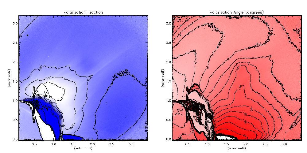
Applying these fomulae to the shifted mean images gives us maps of polarization angle and fraction.

KNAC Paper

The total solar eclipse of June 2001 presented an opportunity to study the inner solar corona from the ground to complement observations from spacecraft. From a site in Lusaka, Zambia, a Williams College team made observations of the corona through filters centered on 3875, 4050, and 4410 angstroms, and three polarizing filters oriented at 45-degree intervals. We made observations of polarization at 2.5 solar radii to compare, by prior arrangement, with observations from the Ultraviolet Coronograph Spectrometer and the Large Aperture Spectroscopic Observatory on the Solar and Heliospheric Observatory. This paper presents maps of polarization intensity and angle off the northwest limb of the moon during the eclipse and discusses future directions for research using these data.

Presentation

Powerpoint presentation for Keck Northeastern Astronomy Consortium 2001 meeting