Lecture 24 (Nov 29)
We started by highlighting one of the steps from the previous lecture: if f(x) tends to a limit as x tends to a, then f is bounded in a neighbourhood of a. We also restated the part of a previous theorem: if f(x) tends to a limit as x tends to a, and g(x) tends to a nonzero limit as x tends to a, and g(x) does not equal zero in some neighbourhood of a, then f(x) / g(x) tends to (lim f) / (lim g) as x tends to a.
We next turned to the squeeze theorem: if f, g, and h are three functions such that f(x) and h(x) tend to the same limit as x tends to a, and such that f(x) ≤ g(x) ≤ h(x) for all x in some neighbourhood of a, then the limit of g(x) as x tends a exists, and equals the limit of f(x). We first proved a special case of this: if 0 ≤ G(x) ≤ H(x) in some neighbourhood of a, and if H(x) tends to 0 as x tends to a, then G(x) tends to 0 as x tends to a. (The proof of this is not hard -- just follow the definition.) Surprisingly, applying this theorem to the choices G = g-f and H = h-f immediately yields the general version of the squeeze theorem.
We then turned to two other types of limits. First, we considered the limit of f(x) as x tends "to infinity". We say f(x) tends to L as x tends to infinity iff for any ε > 0 there exists some number x0 such that |f(x) - L| < ε for all x ≥ x0. Another way to think about this: f(x) is very close to L whenever x is "sufficiently close to infinity".
Second, we looked at left-handed and right-handed limits. We say f(x) approaches L as x tends to a from the left iff for any ε > 0, there exists a δ > 0 such that |f(x) - L| < ε for all x ∈ (a-δ, a). Right-handed limits are the same, except the inequality holds for all x ∈ (a, a+δ).
Finally, we applied the squeeze theorem to prove that sin(x) / x tends to 1 as x tends to 0. (Note that this is ONLY true if x is in radians!) To do this, we considered the unit circle and various triangle sitting inside of it. An easy argument shows comparing the length of a segment to the length of part of the circle shows that sin(x) ≤ x. Constructing a perpendicular to the exterior of the circle, we used similar triangles to prove that the length of this new segment is tan(x). Comparing the area of a certain triangle to the area of the sector of the circle sitting inside the triangle, we proved that x ≤ tan(x). The final step: squeeze theorem FTW!
Lecture 23 (Nov 27)
We spent most of the lecture proving that the limit of a product is the product of the limits. Here, I will only sketch the proof, omitting the details. To make it readable, define Lf to be the limit (as x approaches a) of f(x), and Lg to be the limit (as x approaches a) of g(x). We wish to show that when x is close to (but not equal to) a, f(x)g(x) is close to Lf Lg. We used our ideas from last time to write
Now, |f - Lf| is small in a neighbourhood of a, by definition of Lf. Also, g is bounded in a neighbourhood of a, since the limit of g(x) exists as x approaches a. Thus, the quantity g + Lg is bounded in a neighbourhood of a. Combining these, we see that the first term on the RHS of (*) is small in a neighbourhood of a. A similar argument shows that the second term is also small. Putting this together, we conclude that the LHS is small in a neighbourhood of a, which concludes the proof.
We finished lecture by stating the squeeze theorem, and giving a couple of simple applications.
Lecture 22 (Nov 22)
We started by discussing what it means for a limit to not exist. As an example, we proved (by contradiction) that the function f(x) defined to be 0 when x is irrational and 1 when x is rational, does not tend to a limit as x tends to 3. We then stated a theorem that the limit of a sum of two functions is the sum of the limits of the functions, the limit of the product is the product of the limits, etc. We proved the first statement, and made some headway on proving the second.
Lecture 21 (Nov 20)
We began with a practice problem: prove that x sin(1/x) tends to 0 as x tends to 0. Note that the limit exists, even though the function isn't defined at 0! Next, we considered a more difficult example: we proved that the function (x+1)/x2 tends to 3/4 as x tends to 2. This, and ensuing discussion, took us the rest of the lecture.
Lecture 20 (Nov 15)
We started by setting up some alternative notations for limits. In particular, we used the phrase `f(x) tends to L as x tends to a', which indicates something fundamental about limits: they don't care about the value of f(x) at x = a. The only thing the limit reflects is the behaviour of f(x) for values of x near a. In other words, informally, we say L is the limit of f(x) as x tends to a iff for all x close to a (aside from x = a itself), f(x) is close to L.
This is, of course, unsatisfactory as a definition: what does `close' mean? To get intuition for this, we considered the function h(x) = 3x2 + 1. What is the limit of h(x) as x tends to 2? The answer is clearly 13. But how do you know? We checked that when x is within 1/10 of 2, then h(x) is within 1.23 of 13. Actually, this isn't very convincing evidence that h(x) is close to 13 when x is close to 2. We realized that the natural question is the reverse: can we show that for all x close to 2, h(x) is within 1/100 of 13? Sean showed that the answer is yes: if x is within 1/1230 of 2, then h(x) is within 1/100 of 13. We then asked the more general question: what if rather than asking for h(x) to be within 1/100, we want it to be within ε of 13, where ε is some tiny positive number. Is this true for all x close to 2? After some work, and a trick with taking a minimum, we figured out how to do this.
All this led us to give a formal definition: we say that L is the limit of f(x) as x tends to a iff for every ε > 0, there exists a δ > 0 such that |f(x) - L| < ε whenever 0 < |x - a| < δ. (Note that the condition that 0 < |x - a| is just a fancy way of saying that x does not equal a.) Finally, we proved that the function 1/x tends to 1/3 as x tends to 3.
Lecture 19 (Nov 13)
We began the lecture with a more formal description of one-to-one correspondences. Recall that informally, given two sets A and B, we can compare their sizes by thinking of A as a collection of people, B as a collection of seats (in a theatre, say), and then trying to see if there's a way to seat everyone so that every seat is filled (and no one is left waiting for a seat). If there is such a seating arrangement, we said that A and B are in one-to-one correspondence (alternatively, A and B have the same size).
So how do we formalize this concept? The idea was to use the language of functions. We'll say that f is a one-to-one correspondence between two sets A and B if
(i) f : A → B is a function; and
(ii) for every b in B, there exists a unique a in A such that f(a) = b.
In terms of our informal notions, (i) says that everyone is assigned a seat, and (ii) says that every seat is assigned to precisely one person. We've called such an f a one-to-one correspondence, but there's another fancy name for it: any f satisfying (i) and (ii) is called a bijection from A to B. Finally, we say that A and B have the same size iff there exists a bijection from A to B.
When proving that a function f satisfies (ii), it is often useful to check this in two stages:
(ii)a. for every b in B, there exists an a in A such that f(a) = b; and
(ii)b. if f(a1) = f(a2), then a1 = a2.
In our informal picture, (ii)a. means that every seat is assigned to somebody; (ii)b. means that two different people are never assigned to the same seat. These two conditions also have fancy names: any function f : A → B satisfying (ii)a. is called a surjection; if instead it satisfies (ii)b., f is called an injection. Thus, a function f : A → B is a bijection from A to B iff f is both a surjection and an injection.
I next described an algorithmic way to think about countable sets. Recall that a set A is countably infinite iff A has the same size as ℕ. What this means is that there exists an algorithm for going through the elements of A such that, for any element you pick, the algorithm will get to your element after a finite number of steps. Note the the algorithm comes before your choice of element, i.e. we're not allowed to adjust the algorithm depending on which element you've picked. Thus a set A is uncountable means that, no matter which algorithm you design, there will be some elements of A which the algorithm will never get to. This is quite a strong condition but, as we have seen, it does occasionally arise.
We concluded the lecture by starting to discuss limits. Informally, we say `a function f(x) approaches a limit L as x tends to a' iff whenever x is really close to a, f(x) is really close to L. We did an example with the linear function f(x) = 3x+1; first, we saw that when x is close to 2, f(x) is close to 7, and then we figured out how close x would have to be to 2 in order for f(x) to be at most 1/100 away from 7. The answer was conjectured by Zim, and isn't entirely obvious; however, once you have a guess, verifying that it's right is very easy. This will be a recurring theme, as we'll see on Thursday.
Lecture 18 (Nov 8)
Today we continued our discussion of functions. We started by discussing why the informal definition of function isn't great. The main problem is that it is secretly circular: a function is a rule, which is what? An association... which is a function...
So, instead, we have a different definition for what a function is: it's a set of ordered pairs, satisfying the nice condition that whenever (a,b) and (a,c) belong to the function, then b and c must be equal. Really, this definition just formalizes what the graph of a function is; except that rather than drawing the graph, we list all the points and call the list, the function. We then discussed various examples and non-examples. We concluded the lecture by discussing composition of functions, and noting that functions (with respect to composition) and numbers (with respect to addition) have suspiciously similar properties. This connection is explored more deeply in MATC01 (group theory).
Lecture 17 (Nov 6)
Today we discussed functions. We gave an informal definition: a function f from a set A to another set B is a rule which associates to every element of A an element of B. We introduced some notation for this, and considered many examples (including a the function we called G, which associates to any real number x the number of 7's appearing in the decimal expansion of x, if this is finite; if x has infinitely many 7's, then we defined G(x) to be 2. This is a function, even though nobody knows the value of G(π). We also defined (with some difficulty!) the sine function.
Lecture 16 (Nov 1)
We started the lecture by clarifying the main step in the proof of the nested intervals theorem: we observed that for any natural numbers k and n, we have
Next, we continued discussing sizes of sets. We showed that the union of two countable sets is countable. We also proved that the set of positive rational numbers is countable. Then, somewhat unexpectedly, we proved that the set [0,1] is uncountable!
We concluded the lecture with a discussion of what it means for a function to be continuous. We concluded that it makes sense to discuss continuity at a single point, and identified what this might mean in terms of limits. Next week we will begin a more careful investigation of this important topic.
Lecture 15 (Oct 30)
We started by proving the theorem on nested (closed!) intervals. The first part of this proof caused some confusion; make sure you sort out what's going on in the proof! Next, we began discussing how to compare different infinite sets. Inspired by the movie theatre example, we say that two sets have the same size of there exists a one to one correspondence between them. We showed that ℕ, 2ℕ, and ℤ all have the same size, and finished the lecture by considering whether ℕ and ℚ have the same size.
Lecture 14 (Oct 25)
We reviewed the concepts of upper bound and supremum, and corrected an error (caught by Molly) in our proof that sup (0,1) = 1. Next, we discussed lower bounds and infimum, and briefly sketched why the completeness property implies that inf A exists for any nonempty set A which is bounded below.
We then proved that ℚ is dense in ℝ -- i.e. that between any two (distinct) real numbers there is a rational number. To do this, we began with two positive numbers x and y, with x < y. We wish to show that the interval (x,y) contains a rational number. First, by the Archimedean property, we know that we can stretch the interval to make it longer than a unit interval (i.e. we can find a natural number n s.t. (nx,ny) has length bigger than 1). I next claimed that any interval of length > 1 must contain an integer; we proved this by using the well ordering of ℕ. Thus, we were able to find an integer m with nx < m < ny. This concluded the proof.
After discussing intervals, we proved (up to some details) the nested interval theorem: that if we have a sequence of nested closed, nonempty intervals [an,bn], then there exists a real number which lives in all of these intervals simultaneously. Recall that saying the intervals are nested means that
The idea of the proof is simple. Let A = {an}. The first observation is that A is bounded above (by any one of the bn's). Thus, by completeness, sup A exists. Since sup A is an upper bound of A, we see that
for every n. On the other hand, since bn is an upper bound of A for every n, we see that
for every n (since sup A is the smallest upper bound of A). This concluded the proof. Finally we discussed why it's necessary to assume that all the intervals are closed, by considering the sequence of nested open intervals {(0,1/n) : n∈ℕ}.
Lecture 13 (Oct 23)
We started by recalling the Completeness Property, and restating it in the following (equivalent) form. Given a set A⊆ℝ, define UA to be the set of all upper bounds of A. Moreover, set U∅ := ∅.
The Completeness Property of ℝ: Given A⊆ℝ. If UA ≠ ∅, then UA has a least element.
Note the similarity to the Well-Ordering Property of ℕ.
We next reviewed the proof of the existence of √2 from last lecture. We went over the formal definition of upper bound and supremum of a set, and considered two examples: sup [0,1] and sup (0,1). In both examples, the supremum was equal to 1, but proving this was more difficult in the second case than in the first. The general strategy to proving that the supremum is what you think it should be proceeds in two steps: first, prove that your guess is an upper bound; next, prove that every other upper bound is bigger. One important point from our examples: sup A might live in A, or it might not belong to A!
We concluded the lecture by proving the Archimedean Property. Although the statement is trivial, the proof is subtle -- make sure you understand it!
Lecture 12 (Oct 18)
We started by discussing the definition of ℕ (1∈ℕ, and whenever n∈ℕ, n+1∈ℕ). We defined 2 := 1+1, 3 := 2+1, etc. We next briefly reviewed the triangle inequality and some corollaries.
Next, we attempted to prove that √2 exists. In other words, we tried to prove that there exists some real number α > 0 such that α2 = 2. Here's a sketch of our attempt. Let
and let B denote the set of all upper bounds of A. In other words,
Let α denote the least element of B. (In words: α is the least upper bound of A; it is an upper bound of A, and is smaller than every other upper bound of A. This is also called the supremum of A, or sup A for short. I didn't use this word in lecture, but it's in the book.)
In any event, we have produced some positive real number α. I claim that α2 = 2. To prove this, we first showed that if α2 < 2, then there exists another number which is a little larger than α, but whose square is still less than 2; this contradicts α's being an upper bound of A. Next, we showed that if α2 > 2, then there exists another number which is a little smaller than α, but whose square is still larger than 2; this contradicts α's being the least upper bound of A. By trichotomy, we conclude that α2 must equal 2. So, the square root of 2 exists!
There's only one problem with this proof: how do we know that the set A has a supremum? Actually, this is equivalent to the existence of √2: a little thought shows that sup A exists iff √2 does. Thus, we have not dealing with a problem in the proof, but rather with a philosophical dilemma: either we live in a universe in which √2 does not exist, or we live in a universe in which sets like A have a supremum. This inspired us to make one final assumption about ℝ: the completeness property. This asserts that if a nonempty subset A⊂ℝ has an upper bound, then sup A exists. Note that the supremum may or may not belong to A! We will discuss this further next week.
Lecture 11 (Oct 16)
We started by answering a question of Scott: we proved that if 0 < a < 1, then 0 < a2 < a. I also mentioned that you cannot assume, without proving it yourself, that -1*a = -a. From the properties, all you know about -a is that when you add a to it, you get 0.
Next, we discussed whether there are any sets other than ℝ which satisfy all the algebraic and order properties. One suggestion (due to Slavik) came particularly close: ℤ. This satisfies all the properties aside from one - M4 (multiplicative inverses). Inspired by this near-success, we realized that ℚ satisfies all of our properties. Since we'd earlier proved that √2 ∉ ℚ, we see that the existence of √2 cannot be proved from the algebraic and order properties alone. This might sound crazy at first -- how could √2 not exist? The point is that the symbol √2 is telling us what the number should do rather than what it is. Essentially, when we write √2, we're saying: wouldn't it be nice if there were a number whose square is 2? In the same spirit, we could talk about √ORANGE, the number whose square is ORANGE. As you can see, the existence of such a number -- just as of √2 -- is questionable. Nonetheless, we will be able to prove the existence of √2, once we introduce one more property. In fact, this will be the final property we need to completely define ℝ. We will discuss this property next lecture.
For now, we discussed absolute value. After stating the definition, we talked about the triangle inequality and some corollaries.
Lecture 10 (Oct 11)
Given a statement of the form A ⇒ B, the converse is the statement B ⇒ A; this might be true or false. If both the implication and its converse hold, then we write A ⇔ B. Or in words: A if and only if B. Or, in abbreviated words: A iff B. For example: Well-Ordering of ℕ is true iff Induction is. Another example: ab = 0 iff (a = 0 or b = 0).
The contrapositive of [A ⇒ B] is [(not B) ⇒ (not A)]. An implication and its contrapositive are equivalent -- either both implications are true, or both are false. Sometimes it's more convenient to prove the contrapositive of a statement rather than the statement itself; the example we looked at was: if α is irrational, then √α is as well.
We next discussed the 9 properties A1-A4, M1-M4, D; these don't define the real numbers,
because there are other sets (with weird addition and multiplication) which satisfy all
nine properties! We explored an example in class: the set S={0,1}, where
0 + 0 = 0,
0 + 1 = 1, 1 + 0 = 1, 1 + 1 = 0, 0 x 0 = 0, 0 x 1 = 0, 1 x 0 = 0, 1 x 1 = 1.
Even though I'm using the labels 0 and 1 for the elements
of S, it's better to think of them as abstract objects, rather than as numbers.
We then moved onto the order properties of the real numbers; there exists a subset P of the reals which satisfies three nice properties (0 ∉ P, a ∉ P iff -a ∈ P; a+b and ab are both in P whenever a,b ∈ P). We then defined the symbols >, ≥, <, and ≤ (e.g. a > b iff a - b is in P). We noted that given any two reals, exactly one of a = b, a > b, a < b holds; this property is called trichotomy. I sketched a proof that if a > b, then a+c > b+c for any real number c.
Finally, we proved (up to a lemma) that if a non-negative real number is smaller than every positive real number, then it must be 0. This had a nice implication: 0.99999... = 1.
Lecture 9 (Oct 9)
We began by discussing the difference between figuring out how to prove something, and actually writing the proof. To figure out how to prove a claim, it's often useful to reverse engineer, use intuition, and make logical leaps. But when you write the proof, it should be precise, logical, and easy to follow step by step. As examples, we (re)proved that 0*a = 0 for all real numbers a, and also proved that if ab=0 then one of a or b must be 0. (There were also two extra problems: prove that a+b+c+d is unambiguous for all real a,b,c,d; and prove that a1+a2+a3+...+an is unambiguous.
Next we discussed the dangers of proving things by starting with a statement and manipulating it (5=3 => 0=0). This led us to a discussion of: what is a mathematical statement? (Examples: "5+3=7" is a statement, "Leo's first language was English" is a statement, "MATA31 is awesome" is not a statement.) Given two statements A and B, one can form a new statement: A => B. We saw through examples (some more plausible than others) that the statement A => B is always true UNLESS A is true and B is false.
Lecture 8 (Oct 4)
Click here for the lecture summary.
Midterm 1 (Oct 3)
Click here for midterm solutions.
Lecture 7 (Oct 2)
Today we gave two important applications of strong induction. The first was to prove that any natural number can be written in binary (i.e. as the sum of distinct powers of 2). The second application was to show that any natural number larger than 1 can be decomposed into a product of primes. In both cases, SI made the proofs rather simple. Unlike the Fibonacci example from last lecture, we only needed to check one base case for these examples. (You should makes sure you understand why this suffices here, but not in the Fibonacci example.)
We finished up lecture with the following puzzle. Suppose there are 99 boxes, each containing some number of apples and bananas. Prove that it's possible to pick 50 boxes so that these 50 contain at least half of the total number of apples, and also contain at least half the total number of bananas.
Lecture 6 (Sept 27)
We continued discussing induction. We proved that any 2n x 2n chessboard can be tiled by L-shaped pieces in such a way such that the only square left open is one of the middle four. Actually, this was a corollary of a stronger theorem: that for any such board, and for any given square on the board, we can tile the entire board by L-pieces, with only that one square left untiled.
Next we proved that 1 + 1/22 + 1/32 + ... + 1/n2 < 2 for all natural numbers n. Again, this was a corollary of a stronger theorem: that the sum is actually bounded by 2 - 1/n.
I then showed a ridiculous induction `proof' that n! < 0 for all natural numbers n. The problem was that I forgot to check whether 1 satisfies this.
The next topic was a flexible notion of induction, where one can start at 5 (say) rather than at 1. We followed this up with strong induction (SI), and used SI to prove that the n-th Fibonacci number is less than 2n. A key step in the proof was that we had to check that both 1 and 2 satisfy this hypothesis. Make sure you understand why we need to check two cases, rather than just one as in all the previous problems!
Lecture 5 (Sept 25)
We reviewed induction. We still haven't proved the theorem (coming next lecture!),
but we gave two more applications. First, we proved the curious formula
Lecture 4 (Sept 20)
Recall that we had two proofs that √2 is irrational. In the first,
we defined a set
In the second proof, we worked with a set
Today we quickly proved that A=B. This allows us to restate our two proofs in a way which makes them look very similar:
- Proof 1: If n∈A then n⁄2∈A. Thus A has no least element, and must therefore be empty. QED
- Proof 2: If n∈A then n(√2 - 1)∈A. Thus A has no least element, and must therefore be empty. QED
Well-Ordering Property of ℕ: Every nonempty subset of ℕ has a least element. We noted that this property can fail in other contexts; for example, the set ℚ≥0 of non-negative rationals is not well-ordered.
Next, we wrote down one of the main theorems of the semester: induction. We didn't prove it (yet), but instead, used it to prove the following:
- 1+2+3+...+n = n(n+1)/2
- n < 4n.
Lecture 3 (Sept 18)
Today we spent most of the lecture discussing various notation and clearing up some confusion. We talked about the definition of odd and even numbers, and proved that an odd times an odd gives an odd number. Here's the notation which came up during our discussion:
- ∀ means for all
- ∃ means there exists
- ∅ means the empty set, the set which doesn't contain anything
- A ⊆ B means A is a subset of B (everything which lives in A also lives in B)
We also reconsidered the proof from last time that root 2 is irrational. Precisely, we rewrote the first proof in a way which made it look like the second proof (start with a set consisting of natural numbers, if it's empty we win, otherwise show that it has no smallest element -- which is impossible). We will see (on Thursday) that this point of view leads to some fundamental questions and ideas.
Lecture 2 (Sept 13)
We began by discussing sets and set notation. In particular, a set doesn't care about the order in which its elements appear, e.g. {1,3,5} = {3,1,5}. Also, a set doesn't see repeated elements, e.g. {1,3,3} = {1,3}. We also discussed the notion of equality. If two sets are equal, that means they're not actually two different sets; they're the same set, which we've written down twice. Another (useful) way to describe this is that two sets A and B are equal if they have precisely all the same elements: all the elements of A also live in B, and vice versa.
We next discussed some examples of sets which will come up a lot in this course. The natural numbers, denoted ℕ, is the setNext we discussed circles, the definition of π (it's not 3.1415926, nor is it 22/7), and the discovery that the square-root of 2 is irrational. The entire second half of the lecture was devoted to giving two proofs of this fundamental fact; click below to read them.
Lecture 1 (Sept 11)
We went over the syllabus. After intense negotiations, we decided that
although computers, cameras, e-readers, and phones are not allowed to be used
in the lecture hall, voice recorders and e-dictionaries are permitted.
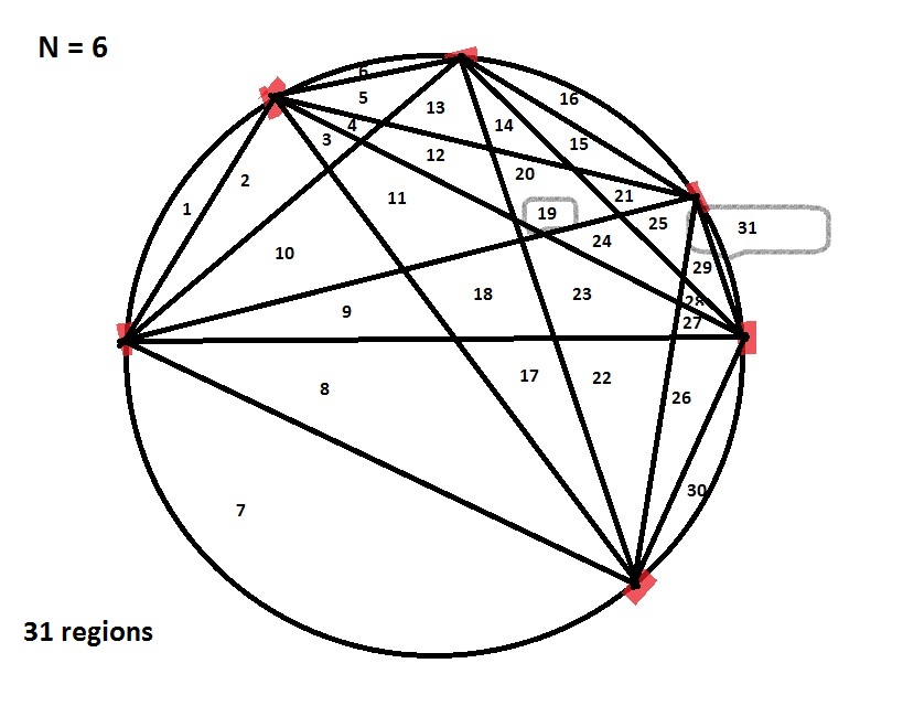
We next discussed the following problem. Given a circle, draw N
points on the circumference, and connect each pair of points with a
straight line. If the N points are random, then we can (and will) assume
that no three lines intersect anywhere in the interior of the circle. (In other
words, every point formed inside the circle is the intersection of exactly two
lines.) Into how
many regions do these lines split the circle? For N = 1, 2, 3, 4, 5, the
answers were (respectively) 1, 2, 4, 8, 16 regions. But for N = 6, the answer
was 31. What's going on?! I left this as a question to ponder for next lecture.
Do not look this up in books / the internet. Where's the fun in
that?
Note: you do not need to bring your textbook to lectures -- the whole point of the lecture is to cover the material in a different way than is done in the book! However, you may find it helpful to bring your textbook to tutorials.