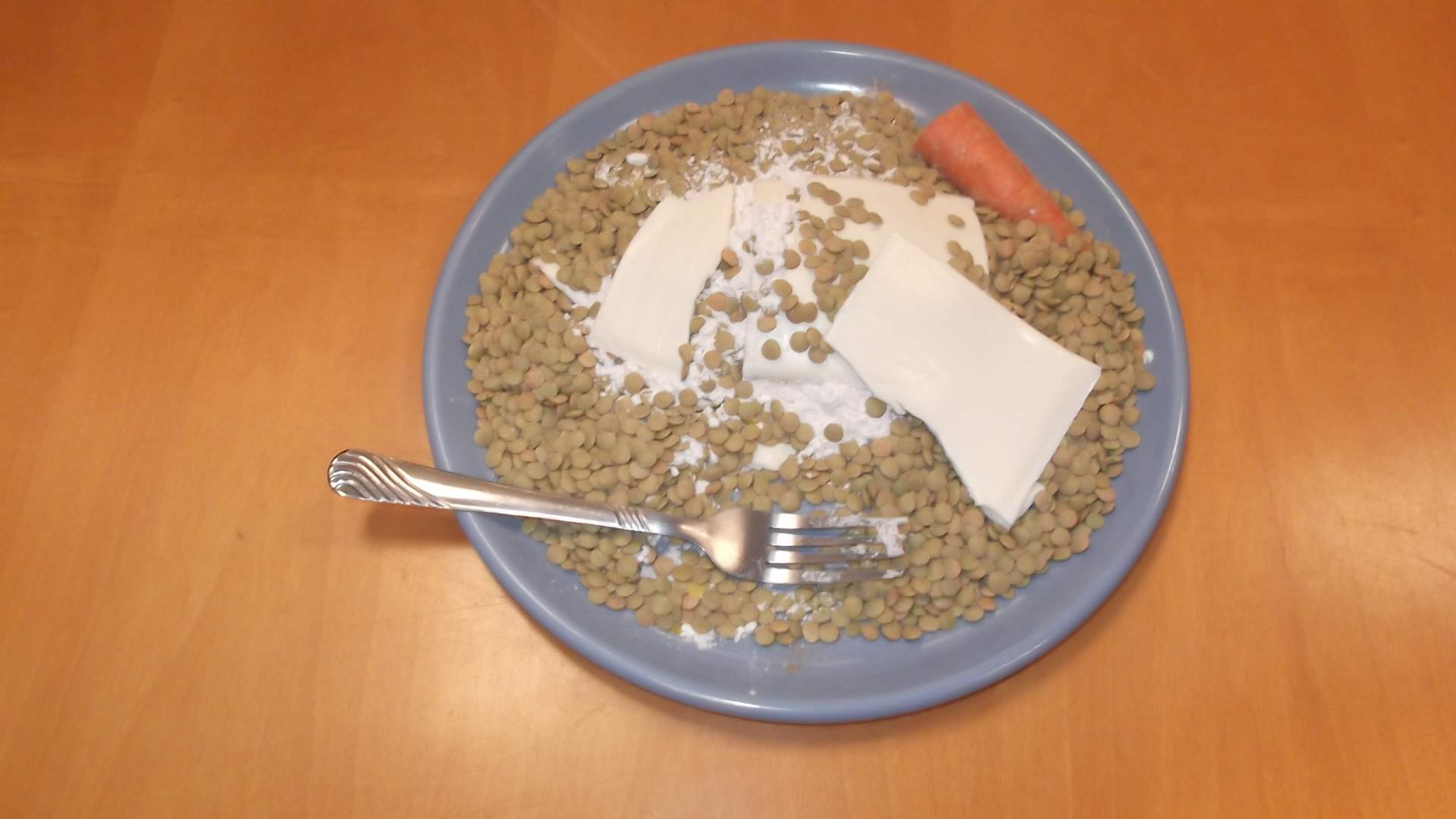
Friday, November 9. Great presentation today on solving the Diet Problem through Peapod (and, as I remarked at the end, the importance of multiobjective programming!).
-
Mmmm.
-
General takeaways (all classes)
MATH 416: Additional comments related to material from the class. If anyone wants to convert this to a blog, let me know. These additional remarks are for your enjoyment, and will not be on homeworks or exams. These are just meant to suggest additional topics worth considering, and I am happy to discuss any of these further.
Wednesday, December 5. Talk today was on machine learning.
Chess: Deep Blue versus Kasparov. Click this article for more.
KKT conditions. I know Kuhn from my Princeton days, and connecting to the lecture the day before he played a key role in getting Nash the nobel prize.
Stacking dominoes is a great example of how we may be unknowingly wearing blinders. A lot of people, when trying to get the greatest overhang with \(n\) dominoes, do a staircase and get close to the harmonic series, with the \(n^{\rm th}\) dominoe overhanging the previous by \(1/n\). This gives an overhang of \(\log n\), but it is possible to do much better.
Here's a Wolfram (Mathematica) demonstration of harmonic stacking.
Here is a brief article explaining why the harmonic series works.
It is possible to do much better than \(\log n\); one can get to order \(n^{1/3}\) but not better; see the great paper by Paterson, Peres (my first college math professor), Thorup, Winkler and Zwick.
A common image for Mathematical Induction is that of following dominoes.
Monday, December 3. Talk today was on game theory and linear programming.
Generalization of rock paper scissors from The Big Bang Theory.
Nash's thesis (original formatting, 27 pages!!!) and an economist's take on it. Here's a discussion on short theses.
Forgot to do the rest of comments on Baker Campell Hausdorf, so here it is:
There is a formula for \(\exp(A) \exp(B)\), the Baker-Campbell-Hausdorff formula, See the Zassenhaus formula for a nice explicit formula for this product. The formula involves the commutator of two matrices, where \([X,Y] = XY - YX \) measures how far \(X\) and \(Y\) are from commuting. The commutator arises throughout the sciences, in particular in quantum mechanics, where the fundamental commutator relation asserts that \([X,P] = i\hbar I\) (\(\hbar\) is planck's constant divided by \(2 \pi\), \(X \)is the position operator and \(P\) is the momentum operator).
Monday, November 26. The talk today on stochastic linear programming talked about recurrences and solving equations, which serves as a nice springboard to exp(At) where A is a square matrix.
Systems of equations are frequently used to model real world problems, as it is quite rare for there to be only one function of interest. If you want to read more about applying math to analyze the Battle of Trafalgar, here is a nice handout (or, even better, I think we could go further and write a nice paper for a general interest journal expanding on the Mathematica program I wrote). The model discussed is very similar to the Lotka-Volterra predator-prey equations (our evolution is quite different, though; this is due to the difference in sign in one of the equations). Understanding these problems is facilitated by knowing some linear algebra. It is also possible to model this problem using a system of difference equations, which can readily be solved with linear algebra. It's worth noting a major drawback of this model, namely that it is entirely deterministic: you specify the initial concentrations of red and blue and we know exactly how many exist at any time. More generally one would want to allow some luck or fluctuations (notice how nicely this now fits in with the stochastic programming). One way to do this is with Markov chains. This leads to more complicated (not surprisingly) but also more realistic models. In particular, you can have different probabilities for one ship hitting another, and given a hit you can have different probabilities for how much damage is done. This can be quite important in the 'real' world. A classic example is the British efforts to sink the German battleship Bismarck in WWII. The Bismarck was superior to all British ships, and threatened to decisively cripple Britain's commerce (ie, the flow of vital war and food supplies to the embattled island). One of the key incidents in the several days battle was a lucky torpedo shot by a British plane which seriously crippled the Bismarck's rudder. See the wikipedia entry for more details on one of the seminal naval engagements of WWII. The point to take away from all this is the need to always be aware of the limitations of one's models. With the power and availability of modern computers, one workaround is to run numerous simulations and get probability windows (ie, 95% of the time we expect a result of the following type to occur). Sometimes we are able to theoretically prove bounds such as these; other times (using Markov chains and Monte Carlo techniques) we numerically approximate these probabilities.
We have \(\exp(z) = 1 + z + z^2/2! + z^3/3! + \cdots\). It is not at all clear from this definition that \(\exp(z) \exp(w) = \exp(z+w)\); this is a statement about the product of two infinite sums equaling a third infinite sum. It is a nice exercise in combinatorics to show that this relation holds for all complex \(z\) and \(w\) (the key step is rearranging the sums and then invoking the binomial theorem).
We showed how we can solve systems of linear differential equations by using matrices: if \(\overrightarrow{v}'(t) = A \overrightarrow{v}(t)\) with initial condition \(\overrightarrow{v}(0)\) then the solution is \(\overrightarrow{v}(t) = e^{At} \overrightarrow{v}(0)\), where \(e^B = I + B + B^2/2! + B^3/3! + \cdots\) for a square matrix \(B\).
While \(\exp(x) \exp(y) = \exp(x+y)\) if \(x\) and \(y\) are real, is this true if \(x\) and \(y\) are square matrices? We'll talk about this next time.
See the notes from Wednesday, October 24th for a proof of many trig formulas from \(e^{i\theta} = \cos\theta + i \sin\theta\).
Monday, November 19.
Today I passed along a fun integral I learned about in Physics 260 (Professor Firk) right before thanksgiving my freshman year. Let \(\int\) be the operator \(\int f\) means \(\int_{t = 0}^x f(t) dt.\) The solution to \( \int f = f - 1 \) (ie, \(\int_{t=0}^x f(t) dt = f(x) - 1\)) is \(f(x) = e^x.\) Let's see why.
\(\int f = f - 1\) ==> \(f - \int f = 1.\)
Thus \((1 - \int) f = 1.\)
Therefore \(f = (1 - \int)^{-1} 1.\)
Using the geometric series expansion \((1-r)^{-1} = 1 + r + r^2 + \cdots\) with \( r = \int\) we find \(f = 1 + \int 1 + \int \int 1 + \int \int \int 1 + \cdots.\)
Now \(\int 1 = \int_{t=0}^{x} 1 dt = x.\)
Now \(\int \int 1 = \int(\int 1) = \int_{t=0}^{x} t dt = x^2/2 = x^2/2!.\)
Now \(\int \int \int 1 = \int(\ \int(\int 1)\ ) = \int_{t = 0}^{x} t^2/2 dt = x^3/3!.\)
We find \(f = f(x) = 1 + x + x^2/2! + x^3/3! + \cdots = e^x.\)
The big question is: can this be made rigorous, and if so how? Happy thanksgiving!
Friday, November 9. Great presentation today on solving the Diet Problem through Peapod (and, as I remarked at the end, the importance of multiobjective programming!).
Mmmm.
Wednesday, November 7. Today's class flowed to being mostly about Stirling, though there was a small amount about how the palindromic condition fixed the Diophantine obstruction, and a bit about how the growth rate of the moments gives information about the density.
We gave a poor mathematician's analysis of the size of n!; the best result is Stirling's formula which gives n! is about n^n e^{-n} sqrt(2 pi n) (1 + error of size 1/12n + ...). We obtained our upper and lower bounds by using the comparison method in calculus (basically the integral test); we could get a better result by using a better summation formula, say Simpson's method or Euler-Maclaurin. We will return to Simpson's method later in the course, as one proof of it involves techniques that lead to the creation of low(er) risk portfolios! Ah, so much that we can do once we learn expectation..... Of course, our analysis above is not for n! but rather log(n!) = log 1 + ... + log n; summifying a problem is a very important technique, and one of the reasons the logarithm shows up so frequently. If you are interested, let me know as this is related to research of mine on Benford's law of digit bias.
It wasn't too hard to get a good upper bound; the lower bound required work. We first just had n < n!, which is quite poor. We then improved that to 2^{n-1} < n!, or more generally eventually c^n < n! for any fixed c. This starts to give a sense of how rapidly n! grows. We then had a major advance when we split the numbers 1, ..., n into two halves, and got 2^{n/2-1} (n/2)^{n/2 - 1}, which gives a lower bound of essentially n^{n/2} = (sqrt(n))^n. While we want n/e, sqrt(n) isn't horrible, and with more work this can be improved.
There are other approaches to proving Stirling; the fact that Gamma(n+1) = n! allows us to use techniques from real analysis / complex analysis to get Stirling by analyzing the integral. This is the Method of Stationary Phase (or the Method of Steepest Descent), very powerful and popular in mathematical physics. See Mathworld for this approach, or page 29 of my handout here.
Instead of proving Stirling's formula, we saw how we could get better and better lower bounds by various techniques. I particulary like the matching games we did. Our first lower bound could be interpreted as dividing the interval in pieces and using the smallest value in each piece; we saw we did much better when we multiplied the largest and smallest value of each block. The reason is we want to minimize the variation in the terms we're bounding: thus 1 2 .. n/2 n/2+1 ... n we match (1,n), (2, n-1), ... and note each product is at least n; this is much better than using 2 for the first n/2-1 and n/2 for the last n/2. For an upper bound, we use each product is less than the middle.
Monday, November 5. The purpose of today's lecture is to highlight how the structure of the matrix ensemble affects the combinatorics. We saw the real symmetric matrices had a matching problem lurking, the number of ways to match 2m objects in pairs. The answer is (2m-1)!!; if each of these matchings contributed equally we'd get a standard normal, but that wasn't the case. Only the adjacent matchings contributed in the limit, leading to the Catalan numbers and the semi-circle.
This suggests the very natural question of trying to tweak the ensemble of real symmetric matrices to increase the contribution of the crossing case while preserving the contribution of the adjacent case. A good suggestion from the class was to also have our matrices symmetric about the anti-diagonal, but it turns out that doesn't add enough. That still leaves us only order N^2; we need to have a lot more symmetry.
We looked at Toeplitz ensembles. These matrices have a lot of very nice properties; for us, what matters is they are constant along diagonals. We thus have only on the order of N independent entries on our matrix, not N^2. It is thus far more likely to have a `collision' and have an a_ij equal an a_mn.
We analyzed the fourth moment in detail. We saw there was no extra contribution to the adjacent case from matching along the same diagonal; in Wednesday's class we'll see the matchings must be on the reflected diagonal. There is an increase in the crossing case; these now contribute, but there's an obstruction to the Diophantine equation and it is not quite a full contribution. This can be fixed by looking at circulant or palindromic Toepitz matrices (see my paper on Palindromic Toeplitz, which leads to a proof of a central limit theorem).
I've supervised several papers with students on these ensembles over the years. The first paper has the convergence details and general history of the problem, which is then tweaked in subsequent papers.
Friday, November 2. We finally finished the semi-circle calculation (or as much as we'll do for the real symmetric calculation). We'll have one more lecture on random matrix theory on Monday, and then move to a new topic (hopefully some of you will be ready to present by Wednesday -- remember you're supposed to email me your target dates!).
We showed that while the method of divine inspiration failed for solving the Catalan numbers, the generating function approach worked very well. We introduced the notion of convolution, and showed why it is so important in probability.
We were fortunate that our recurrence relation has a nice combinatorial interpretation; this is what allowed us to get a nice closed form expression for the generating function. We were left with a cubic to solve. Any linear equation (ax+b=0), quadratic (ax^2+bx+c=0), cubic (ax^3+bx^2+cx+d=0) or quartic (ax^4+bx^3+cx^2+dx+e=0) has a formula for the roots in terms of the coefficients of the polynomials; this fails for polynomials of degree 5 and higher (the Abel-Ruffini Theorem; see also Galois). There is an explicit, closed form expression for the three roots of a cubic; while it may not be as simple as the quadratic formula, it does the job (and is better than the quartic formula). Interestingly, if you look at x3 - 15x - 4 = 0, the aforementioned method yields (2 + 11i)1/3 + (2-11i)1/3. It isn't at all obvious, but algebra will show that this does in fact equal 4! As you continue further and further in mathematics, the complex numbers play a larger and larger role.
We needed to Taylor expans sqrt(1 - 4x). This is known as Newton's generalized binomial theorem. It took awhile but we were able to manipulate the expressions and get a nice binomial coefficient pop out. This is one of the hardest parts of the analysis, manipulating the expressions / multiplying by 1 / adding 0 cleverly and recognizing something nice.
Wednesday, October 31. The calculation of the contribution of the matchings to the even moments proceeds similarly to that of the odd moments, with one difference. Now there is a term that contributes (not surprisingly, as otherwise all the moments would vanish!). The same argument shows there are no contributions in the limit if we have any triple or higher matching, and thus it all comes down to what happens when things are matched in pairs.
The largest the 2m-th moment can be is (2m-1)!!, where !! is the double factorial (the Wikipedia entry mentions some occurrences of it). It's nice to see a combinatorial interpretation to the moments of the standard normal / Gaussian / bell curve.
We computed the 2nd and 4th moments. The second moment is straightforward -- whoops, I just realized I used a non-standard normalization in class. It should be division by 2^k N^{k/2+ 1}, not 2^{k/2} N^{k/2 + 1}; I had the wrong power of 2. It's not a big deal, just changes it from a semi-circle to a semi-ellipse. The fourth moment is more interesting. We see that it's not enough to be matched in pairs; there are situations where we can be matched in pairs and contribute, but have so few realizations of that matching that in the limit as N --> oo we get no net contribution.
For real symmetric matrices, the only matchings that contribute in the limit are when items are matched in pairs with no crossing. The number of such matchings are the Catalan numbers. Not surprisingly, these special numbers have many uses and a variety of applications; see Koshy's book for example. See also the Mathworld article on Catalan numbers and the OEIS entry A000108. We will discuss these in greater detail on Friday. We'll be able to find formulas for these numbers by using a generating functions and Taylor series expansions (for more on Taylor series, see the entries from Wednesday, October 24).
We were able to get a very nice recursion formula for the Catalan numbers by doing some clever combinatorics. We conditioned on the first time we hit the diagonal line, and used that to break our paths into distinct classes. This is a very common and important technique.
Finally, we talked a bit about why dividing by sqrt(N) for normalizing the eigenvalues is so important. If we divide by a higher power of N then all the mass concentrates at 0 in the limit; if we divide by less it spreads out and there's no nice limit. If you've seen Hausdorff dimensions, this critical exponent is quite similar. If you haven't seen this before, I strongly urge you to read this Wikipedia link. Click here for a nice list of dimensions of various objects.
Monday, October 29. In previous days we discussed the Eigenvalue Trace Lemma and how we can use it to find the moments of a distribution; today we did the nitty gritty calculation.
While the Eigenvalue Trace Formula is an important start, it's just a start. It allows us to replace what we want to study (the eigenvalues) with something we can study (the matrix elements); however, this exchange would be useless if we didn't have a good averaging formula. For real symmetric matrices it boils down to counting how many ways we can match elements in pairs, where a_ij = a_mn if and only if (i,j) = (m,n) or (i,j) = (n,m).
The argument today was a bit involved. It's worth thinking about it step by step and seeing what's going on. Again, I am *not* holding you responsible for reproducing these arguments, but as math majors you should be aware of long, involved arguments like this.
Step 1: Eigenvalue Trace Formula: The average kth moment is M_{k,N} = Integral ... Integral Sum_{i_1, ..., i_k = 1 to N} a_{i1,i2} ... a_{ik,i1} p(a_{11}) ... p(a_{NN}) da_{11} ... da_{NN} / 2^(k/2) N^{k/2+1}. We study k = 2m+1 odd.
Step 2: There are N^k possible tuples for the product of the a_ij's; as we only divide by N^{k/2+1} there is a potential for an enormous contribution. We must figure out how large we expect the contribution to be as N --> oo.
Step 3: We want to show that in the limit as N --> oo this agrees with the moments of the semi-circle. As the semi-circle density is zero if |x| > 1, the k-th moment of the normalized semi-circle is at most 1 and thus is bounded, independent of N.
Step 4: If any a_ij is unmatched in the expansion above, the contribution is zero. This is because the a_ij's are independently drawn from a distribution p with mean zero and variance 1. If an a_ij occurs to the first power, it leads to an integral Int_{-oo to oo} a_ij p(a_ij) da_ij, which is zero. Thus the a_ij's are matched at least in pairs.
Step 5: The contribution from any product of k of the a_ij's is at most max_{1 <= i <= k} p_i^k, where p_i is the i-th moment of p (the higher moments are all assumed to be finite). The reason is if we have a matching of r objects together, it contributes int_{-oo to oo} a^r p(a) da, which is the r-th moment. This is a bit overkill, as the true value is the product of the moments from matching, but all we care about are finding upper bounds depending on k and not on N. Let's write B_k for this bound.
Step 6. We look at the different matching configurations: we could have (2, 2, ..., 2, 3), or (2, 2, ..., 2, 3, 2), .... What matters is the number of such configurations is a function of k and NOT of N. This makes sense: we have to match k objects such that things are matched in at least pairs. Let's call the number of such configurations C_k.
Step 7: We look at how many ways there are to realize a given configuration. If a_ij is matched with a_mn then either i=m and j=n or i=n and j=m (ie, there are at most 2 ways). Every time we have a match we lose a degree of freedom except for the last matching. This is what I missed in class; the last term has to be matched with something earlier, and both of its indices are thus already known (the i_k from immediately before and the i_1 as that was the first). Thus we start with k=2m+1 indices. There are two free indices in the first object a_{i1 i2}, and then we lose a degree of freedom for all but the last matching; as there are m+1 matchings (worse case is when we have (2, 2, ..., 2, 3), and all in a matching of 2 save for one triple; there are m-1 matches of 2 and 1 match of 3 for a total of m+1 matches since the one match of 3 counts twice). We are left with 2m+1 - m = m+1 degrees of freedom. For each we have at most 2 possible choices in a matching, for a total of 2^k N^{m+1}.
Step 8: We put things together now: the total contribution is at most 2^k N^{m+1} * C_k * B_k, we divide by 2^{k/2} N^{k/2+1} = 2^{k/2} N^{m+1+1/2}, which gives us Const(k) / N^{1/2}, which tends to 0 as N --> oo.
It's worth looking at the proof again. We broke the analysis into stages, overestimating time and time again. It's fine to do so as long as, at the end of the day, our bounds suffice. If they're too crude we then have to revisit our calculations, but since we have something that tends to zero we're fine.
Friday, October 26. We continued our linear algebra review, revisiting old results from a fresh perspective, seeing how they tie in to random matrix theory.
We began with a study of the Eigenvalue Trace Lemma, and the subsidiary results needed to prove it. We first handled simpler cases, namely A is diagonal or upper triangular, and then saw that we could handle the general case by reducing to these cases. We proved several nice theorems along the line, most importantly if Q is orthogonal then A and Q^T A Q have the same eigenvalues. The proof used the characteristic polynomial det(A - lambda I) (this is good for theoretical investigations, just not for numerical ones), and we multiplied by 1 twice in the proof. It's natural to have a result like this: the eigenvalues are a fundamental property of the transformation, and do not depend on the choice of directions.
While the trace is independent of the choice of axes, the sum of all matrix elements is not. Thus, there are some quantities can change as we change coordinate systems. You want to find the quantities that are invariant (read this link for more), that don't depend on the choice of basis. These will be very important, and will contain a lot of information.
In our proofs we used Det(AB) = Det(A) Det(B); this is similar to homomorphisms from algebra, or in a sense hash functions in cryptography and elsewhere. Many matrices collapse to the same value. What's nice is that the determinant is a real number, and thus we have commutivity of this product.
We proved the trace is cyclic by expanding the definition and choosing good labels for the indices, and then using commutivity of multiplication. We could, as noted in class, prove Tr(XY) = Tr(YX) and then let X=A and Y=BC. It's good to see many proofs. The danger is then thinking the trace is commutative, and going from Tr(ABC) to Tr(BAC), which in general fails.
We could have proved the eigenvalue trace lemma by expanding out Det(A - lambda I) and looking at coefficients. Another nice item to see is the Cayley-Hamilton Theorem.
Wednesday, October 24. The slides are online here (click on the classical random matrix theory section).
One of the first questions that arises in the subject is the correct scale to study the eigenvalues. This is a great problem, and is an easy consequence of the Central Limit Theorem and the Eigenvalue Trace Lemma. The power of the Eigenvalue Trace Lemma is that it converts information we have (on the matrix elements) to information on what we want (the eigenvalues). Trace lemmas are powerful and important to find in mathematics, as they form a bridge between subjects. You can view these as another example of the duality principle, converting from one object to another. For me in my research, Poisson Summation is another great example.
Numerous problems can be described by the eigenvalues of matrices, ranging from properties of graphs to bus routes in Mexico.
A lot of random matrix theory boils down to combinatorics. Particularly important objects for us will be the Catalan numbers. We'll talk more on this later.
See the article by Brian Hayes for a bit more of the history of the connection between Random Matrix Theory and Number Theory (though there are a few math mistakes in the article!).
The moments of a distribution are important, and encode a lot of information about them. Hamburger's theorem is a favorite of mine (both in terms of utility and nomenclature).
A major part of today's lecture was trying to figure out the correct scale to study something. We talked about the inner or dot product of functions, and used finite dimensional vector space analogues to motivate the integral dot product for continuous functions. We saw the need to put in a factor of 1/N or 1/(N+1) in order to have convergence to the Riemann integral.
Another example of finding the correct scale is the Dirac delta functional. This leads to the notion of an approximation to the identity, which is what we did with our delta_M(x) functions.
The first step in any investigation is to figure out what questions to ask. After awhile, we got the two standard ones: (1) does the Taylor series exist (or for what x does it converge and equal the original function), and (2) is the Taylor series unique? The answers were surprising; a Taylor series must converge at the expansion point, but it's possible to onlyconverge there; it's also possible for two different, infinitely differentiable functions to have the same Taylor series!
Analysis is hard. The function f(x) = exp(-1/x2) if x is not zero and 0 otherwise has all of its derivatives vanish at 0, but its Taylor series agrees with the original function only at x=0 (which is nothing to be proud of!). Complex analysis is quite different; there if a function is complex differentiable once then it is infinitely complex differentiable, and it equals its Taylor series in a neighborhood of the point. This fact is one reason why we frequently use characteristic functions instead of generating or moment generating functions (which we'll cover later in the semester). We also discussed the similarities between how Taylor coefficients uniquely determine a nice function and how moments uniquely determine a nice probability distribution. It is sadly not the case that a sequence of moments uniquely determines a probability distribution; fortunately in many applications some additional conditions will hold for our function which will ensure uniqueness. For the non-uniqueness of Taylor series, the standard example to use is f(x) = exp(-1/x^2) if x is not zero and 0 otherwise. To compute the derivatives at 0 we use the definition of the derivative and L'Hopital's rule. We find all the derivatives are zero at zero; however, our function is only zero at zero. We will see analogues of this example when we study the proof of the Central Limit Theorem.
Friday, October 19. While there is a lot more that can be done on linear programming, one of the goals of this course is to give you a sense of what's out there mathematically, and thus today we shifted gears to random matrix theory (RMT).
While the origins of the subject go back to statistics, Random Matrix Theory gained popularity due to its predictive power in nuclear physics and number theory. For a description of the nuclear physics origins, basic results and connections to number theory, see chapter 15 of my book An Invitation to Modern Number Theory.
Today's class became a discussion of orthogonal matrices, triangular matrices, and the spectral theorem for real symmetric matrices.
Wednesday, October 17. In general, the optimal solution where the inputs are integers need not be near the optimal solution when the inputs are real.
We started with one of my favorite problems, given S = a1 + ... + a_n with each a_i a positive integer and the goal to maximize the product of the a_i. We quickly see the optimal is when each a_i is 2 or 3, and since 2*2*2 < 3*3 we want 3s over 2s. We converted to a real problem and assumed there were n summands, each a real number. We got a function defined on the integers to maximize, replaced it with a function defined on the reals so calculus would be applicable. We then curve sketched and saw the function was increasing to its maximum and decreasing past it, so the optimal integer soln was either to the left or right of the optimal real soln (here optimal soln is referring to the number of summands). It's unusual to be this fortunate.
We had to maximize a1 * ... * a_n given a_1 + ... + a_n = S and each a_i > 0. We can do this with Lagrange multipliers, or since each a_i in [1, S] we can appeal to the n=2 case because a real continuous function on a compact set attains its max and min. What is nice is that this existence result from real analysis improves to being constructive; if we were at the optimal point and all coordinates were not equal, we could simply replace two of them with the average and improve the product.
A nice application of this problem is that for disk storage (see radix economy), base 3 has advantages over base 2, though base 2 has the very fast binary search. Another nice example of base 3 occurs with the Cantor set.
We then turned to the knapsack problem, and saw that optimal integer solns need not be anywhere near optimal real solns. One issue, not addressed in the book, is actually fitting the objects into the knapsack. We mentioned that one way to do this is to create a lattice, keeping track of the orientation of how each piece is placed inside. The constraints are quite similar to those from the chess problems we studied. We talked a bit about the sphere packing problem (and the three-dimensional version, the Kepler conjecture, with some of the key papers / ideas described here).
Monday, October 15. Today's class had two great themes: comparing the seemingly comparable, and weights. The two turn out to be related, and in fact we often use weights to facilitate such comparisons, but of course weights have a far greater reach and importance.
We started by talking about having a complete order for complex numbers. We tried using norms, but that collapsed several numbers that were initially unequal to being equal. We tried the lexicographic ordering, which has a lot of appealing properties. Unfortunately, it cannot work. We proved there is no way to have an ordering that satisfies the trichotomy property (exactly one of x < y, x = y, x > y holds for any two x and y) and a rescaling property (if a < b and c > 0 then ac < bc). We showed there is no such ordering by looking at a special element, i. If i > 0 we got a contradiction, and we got one if i < 0. It's natural (or should be!) to look at such a special element. We can't just look at the real numbers, as we know an ordering exists there. The simplest new element to look at is i, the square-root of -1. (For fun, what is i^i?).
For more on this argument, click here. What is so important about this, and what makes this worth time in class (over doing the algebra in the chapter, which you can read) is that we can't always do what we want on our wish-list. We can't compare two complex numbers in such a way as to preserve the scaling property. It's thus worth thinking about the limitations in whatever you're doing before you start your work.
We spent a lot of time talking about weights. They allow us to compare apples and oranges, but it's often not clear what the correct choices should be. Different people can legitimately come up with different assignments, leading to different answers. We talked a bit about weights in mathematics. I used counting primes as an example. We started with Euclid's proof (see the comments from Wednesday, October 10 for more details). We then moved to the Riemann zeta function, zeta(s), one of the most important functions in all of mathematics. It falls into the category of a generating function, and allows us to pass from local information to a global object, from which we can extract a lot of information.
Friday, October 12. We finished our discussion of linear recurrence relations. It's hard to do such a vast topic justice in just one or two lectures, but we can at least get a feel for what we can do, and where they arise.
We first used the method of divine inspiration to show that our guess of a_n = r^n works, so long as r satisfies a polynomial associated to the recurrence. This is called the characteristic equation. We spent a lot of time talking about how to solve linear recurrences. If the roots are distinct it's fine; if the roots are repeated it's more complicated. By looking at the special sequence a_{n+2} = 2 a_{n+1} - a_n with initial values 0, 1 we got 0, 1, 2, 3, 4, 5, ...; using initial values of 1, 1 yielded 1, 1, 1, 1, 1, .... The characteristic equation is r^2 - 2r + 1, which has the repeated root of 1. This suggests that the two solutions might be r^n and n r^n (this is the same as n r^{n-1}, as the 1/r can be absorbed by the constant). We then talked about how to `see' that this is a reasonable second solution by looking at clever combinations. We tweaked the solutions a bit and got to a new characteristic equation with distinct roots r1 and r2, and tried solutions (r1^n + r2^n)/(r1+r2) and (r1^n - r2^n)/(r1-r2). As the tweak tends to zero, the roots converge to r and the first solution becomes r^{n-1} while the second becomes n r^{n-1}. There were lots of ways to see this, ranging from factorization (pulling out an r1-r2 from the numerator, my favorite), to interpreting this as approximating the slope of the tangent line of f(r) = r^n, to L'Hopital's rule. The reason I harped so much on this is that frequently it is very hard to solve a problem in mathematics, but if we have a feel for what the solution is like, that can help narrow our search (another example of this, from differential equations, is the Method of Variation of Parameters).
There are lots of applications of linear recurrence relations, and more generally linear differential equations, and even more generally recurrence and differential equations. Unfortunately in general it is impossible to obtain closed form solutions.
Systems of equations are frequently used to model real world problems, as it is quite rare for there to be only one function of interest. A fun example is applying math to analyze the Battle of Trafalgar. Lancaster has a nice paper (click here for his paper) (here is a Mathematica program I wrote to analyze it). The model is very similar to the Lotka-Volterra predator-prey equations (our evolution is quite different, though; this is due to the difference in sign in one of the equations). Understanding these problems is facilitated by knowing some linear algebra. It is also possible to model this problem using a system of difference equations, which can readily be solved with linear algebra. Finally, it's worth noting a major drawback of this model, namely that it is entirely deterministic: you specify the initial concentrations of red and blue and we know exactly how many exist at any time. More generally one would want to allow some luck or fluctuations; one way to do this is with Markov chains. This leads to more complicated (not surprisingly) but also more realistic models. In particular, you can have different probabilities for one ship hitting another, and given a hit you can have different probabilities for how much damage is done. This can be quite important in the 'real' world. A classic example is the British efforts to sink the German battleship Bismarck in WWII. The Bismarck was superior to all British ships, and threatened to decisively cripple Britain's commerce (ie, the flow of vital war and food supplies to the embattled island). One of the key incidents in the several days battle was a lucky torpedo shot by a British plane which seriously crippled the Bismarck's rudder. See the wikipedia entry for more details on one of the seminal naval engagements of WWII. The point to take away from all this is the need to always be aware of the limitations of one's models. With the power and availability of modern computers, one workaround is to run numerous simulations and get probability windows (ie, 95% of the time we expect a result of the following type to occur). Sometimes we are able to theoretically prove bounds such as these; other times (using Markov chains and Monte Carlo techniques) we numerically approximate these probabilities.
We proved Binet's formula several ways. The first was through divine inspiration, the second through generating functions and partial fractions. Generating functions occur in a variety of problems; there are many applications near and dear to me in number theory (such as attacking the Goldbach or Twin Prime Problem via the Circle Method). The great utility of Binet's formula is we can jump to any Fibonacci number without having to compute all the intermediate ones. Even though it might be hard to work with such large numbers, we can jump to the trillionth (and if we take logarithms then we can specify it quite well).
Our original motivation for difference equations were the Fibonacci numbers; here's the fun video I showed. A very nice application is to analyzing betting strategies for roulette; here's a video I did with OIT on the subject.
Wednesday, October 10. OK, I lied a bit last Wednesday. We hadn't finished linearization; while we handled binary operators like IF-THEN, AND, OR, ... and functions such as MAX/MIN, ABS, TRUNCATION, there's more that can be linearized. We showed how to linearize polynomials in products of binary indicator variables by using IF-THEN and binary variables. It turns out that we can linearize general polynomials as well -- think about how to convert a general integer random variable in terms of binary integer variables. The issue, of course, is the cost to the run-time in doing this.
Just because we can solve something doesn't mean we can solve it quickly / efficiently. A classic example is the (binary) Goldbach problem, which states that every sufficiently large even number can be written as a sum of two primes (we believe that sufficiently large means 4 or greater). We can use generating functions to write down an integral whose value corresponds to the number of ways of writing 2n as a sum of two primes; unfortunately we cannot evaluate this integral well enough (in general) to show it is non-zero! This indicates that just because we can write down an expression for a problem does not mean it's useful.
It is possible to get so caught up in reductions and compactifications that the resulting equation hides all meaning. A terrific example is the great physicist Richard Feynman's reduction of all of physics to one equation, U = 0, where U represents the unworldliness of the universe. Suffice it to say, reducing all of physics to this one equation does not make it easier to solve physics problems / understand physics (though, of course, sometimes good notation does assist us in looking at things the right way).
We moved from talking about generating functions in the Goldbach problem (which we discussed as an example of how just because we can write something down does not mean we can solve it) to solving recurrence relations (which are discrete versions of differential equations). We'll see on Friday that generating functions appear here too.
We analyzed a population problem involving the number of pairs of whales of various ages at any time (v_{n+1} = A v_n where A is a Leslie matrix). We first modeled this with a simple constant coefficient system of difference equations, which we can solve completely. We then discussed the problems with such a model, and possible generalizations that would address these issues. For more details, see the two models described in my notes here. Interestingly, there is a connection between the generalized model and random matrix theory!
There are many ways to find solutions linear constant coefficient homogenous difference or differential equations. We saw one approach involving powers of matrices. Another is the Method of Divine Inspiration. I've written up some notes about this method.
In studying difference equations we saw how linear algebra can be useful; in particular, the need to evaluate large powers of a matrix quickly. This is known as fast exponentiation, and the ability to do this (both for matrices as well as regular numbers) is extremely important. For example, one's first instinct is to say we need 100 (or 99) multiplications to evaluate x^100, but it is possible to do this in just 8: x*x, x^2 * x^2, x^4 * x^4, x^8 * x^8, x^16 * x^16, x^32 * x^32, x^64 * x^32 * x^4. The key observation is using the base 2 expansion of 100; this idea is one of the reasons RSA encryption is feasible. For more details, see Chapter 1 of my book,http://press.princeton.edu/chapters/s8220.pdf (especially Sections 1.1 and 1.2.1). Quite often in mathematics we have algorithms to solve problems that are not feasible in practice, and finding efficient ways of computing quantities is a big (and important) industry. Another great example of where we know the solution exists but have trouble finding it is Euclid's proof of the infinitude of primes. Euclid argued that there must be infinitely many primes as follows: Assume not, and thus let p_1, ..., p_n be all the primes. Consider the product p_1 * ... * p_n + 1; either that number is prime, or it is divisible by a prime p. This prime p cannot be any of p_1, ..., p_n, as each p_i leaves remainder 1. Thus there are infinitely many primes, and we denote this new prime p by p_{n+1}. Lather, rinse, repeat. Keep doing this and we'll get an infinite list of primes. OK, great. This shows there are infinitely many. What can we say about the sequence of primes constructed? Does it contain all the primes? Do we know which primes are in the list and when? Is it easy to compute the terms? Euclid's method leads to the following sequence of primes: 2, 3, 7, 43, 13, 53, 5, 6221671, 38709183810571, 139, 2801, 11, 17, 5471, 52662739, 23003, 30693651606209, 37, 1741, 1313797957, 887, 71, 7127, 109, 23, 97, 159227, 643679794963466223081509857, 103, 1079990819, 9539, 3143065813, 29, 3847, 89, 19, 577, 223, 139703, 457, 9649, 61, 4357.... (Remember how we generated the sequence. We started with p_1 = 2, the first prime. We apply Euclid's argument and consider 2+1; this is the prime 3 so we set p_2 = 3. We apply Euclid's argument and now have 2*3+1 = 7, which is prime, and set p_3 = 7. We apply Euclid's argument again and have 2*3*7+1 = 43, which is prime and set p_4 = 43. Now things get interesting: we apply Euclid's argument and obtain 2*3*7*43 + 1 = 1807 = 13*139, and set p_5 = 13.) This is a great sequence to think about, but a computational nightmare to enumerate! I downloaded these terms from the Online Encyclopedia of Integer Sequences (homepage is http://oeis.org/ and the page for our sequence is http://oeis.org/A000945). You can enter the first few terms of an integer sequence, and it will list whatever sequences it knows that start this way, provide history, generating functions, connections to parts of mathematics, .... This is a GREAT website to know if you want to continue in mathematics. There have been several times I've computed the first few terms of a problem, looked up what the future terms could be (and thus had a formula to start the induction).
Wednesday, October 3. We finished our discussion of linearization. We showed an impressive number of functions / expressions that might initially seem outside the realm of linear programming can in fact be done linearly through the introduction of binary integer variables. Unfortunately, this means that if the original problem were solvable by the simplex method (haivng real variables and constraints), this new system would convert us to an integer programming problem, which has a higher complexity.
We used truth tables to convert an IF-THEN statement to an INCLUSIVE OR. Read about Boolean algebras for more on this important topic. You've seen this at various points in your math career; sometimes it's easier to attack the contrapositive rather than the original statement.
A major theme of today's lecture was building complicated functions out of simpler ones. In the end, we could get trunctations, maximum and minimums, and absolute values from IF-THEN and other operations. This shows that we can build complicated functions out of simpler pieces.
In calculus the absolute value function wreaks havoc, as it is not differentiable. In linear programming it's effect is far less, as we can essentially linearize it (at the cost of introducing binary indicator variables). This led to conversations on how to measure errors. The Method of Least Squares is one of my favorites in statistics (click here for the Wikipedia page, and click here for my notes). The Method of Least Squares is a great way to find best fit parameters. Given a hypothetical relationship y = a x + b, we observe values of y for different choices of x, say (x1, y1), (x2, y2), (x3, y3) and so on. We then need to find a way to quantify the error. It's natural to look at the observed value of y minus the predicted value of y; thus it is natural that the error should be Sum_{i=1 to n} h(yi - (a xi + b)) for some function h. What is a good choice? We could try h(u) = u, but this leads to sums of signed errors (positive and negative), and thus we could have many errors that are large in magnitude canceling out. The next choice is h(u) = |u|; while this is a good choice, it is not analytically tractable as the absolute value function is not differentiable. We thus use h(u) = u2; though this assigns more weight to large errors, it does lead to a differentiable function, and thus the techniques of calculus are applicable. We end up with a very nice, closed form expression for the best fit values of the parameters.
It is possible to get so caught up in reductions and compactifications that the resulting equation hides all meaning. A terrific example is the great physicist Richard Feynman's reduction of all of physics to one equation, U = 0, where U represents the unworldliness of the universe. Suffice it to say, reducing all of physics to this one equation does not make it easier to solve physics problems / understand physics (though, of course, sometimes good notation does assist us in looking at things the right way). I'm mentioning this here as what he does involves measuring errors by squaring, the topic discussed a moment ago. For each physics equation look at the square of the left hand side minus the right hand side, then sum everything and call that U. Thus one term is say (F - ma)^2, and thus we see that the only way U = 0 is if each summand is zero, and thus each physics equation must hold.
Monday, October 1. We discussed the Strassen algorithm (see also the Mathworld entry here, which I think is a bit more readable), and saw that it led to great savings in run-time for matrix multiplication, moving it from an order N^3 operation (for N x N matrices) to order N^(log_2 7) =approx= N^2.8074. There are better algorithms, as well as related algorithms for other common operations (see the comments from Friday's lecture). Our other item for today was linearizing non-linear terms for linear programming. We need to do this in order to increase the reach of the subject.
Friday, September 28. There are many processes in mathematics that run in far less time than they appear. The Euclidean algorithm is a terrific example. It runs far faster than expected; it doesn't take min(x,y) steps but rather 2 log(min(x,y)). It's a beautiful example of a major theme of the course, the need to do things fast. The other topic was linearization non-linear terms. This was a major theme of calculus (Newton's method is a terrific example).
Wednesday, September 26. The Simplex Method allows us to solve the standard linear programming problem. There were a lot of clever ideas in the proof. The first was that we used Phase II to prove Phase I and then used Phase I to prove Phase II; this seems illegal as Phase II requires Phase I, but fortunately it isn't. The idea is if we can find a solution to a related problem, we can pass from that to a solution to the problem we care about. This is somewhat similar to the auxiliary lines that appear in geometry proofs; the difficulty is figuring out where to draw them. We needed to pass from our original problem to a related one. To use Phase II we needed a function to optimize, and we had to figure out what that should be. A little thought shows it can't involve c^T x. Why? The goal is to find a feasible solution to the original problem right now; only later will we worry about finding an optimal solution. Thus, c^T x can't be involved yet, as that has no bearing on whether or not the original problem has a feasible solution.
We talked about tic-tac-toe today as a counting problem: how many `distinct' games are there. We are willing to consider games that are the same under rotation or reflection as the same game; see http://www.btinternet.com/~se16/hgb/tictactoe.htm for a nice analysis, or see the image here for optimal strategy.
Probably the most famous movie occurrence of tic-tac-toe is from Wargames; the clip is here (the entire movie is online here, start around 1:44:17; this was a classic movie from my childhood).
The math conundrum this month involves tic-tac-toe and a fun generalization: First Conundrum: Tic-Tac-Toe. Consider ‘Russian Doll’ tic-tac-toe. Each person has two large, two medium and two small pieces; the large can swallow any medium or small, the medium can swallow any small. If someone gets 3 in a row they win, else it’s a tie. If blue goes first, do they have a winning strategy (can they make sure that they win, no matter how orange responds)? If not, can blue at least ensure that they do no worse than tie? Feel free to come to my office (Bronfman 202) to ‘test’ your theories on a board. Email solns to sjm1 AT williams.edu by Oct 1, 2012.